Marketing Analytics

Data-Driven Techniques with Microsoft Excel

Wayne L. Winston

• Publisher: Wiley
• Year: 2014
• ISBN:
  9781118417300
• Edition: 1
• Topic: Computer Science
• Subtopic: Data Mining
• Index: Computer Science

Helping tech-savvy marketers and data analysts solve real-world business problems with Excel

Using data-driven business analytics to understand customers and improve results is a great idea in theory, but in today's busy offices, marketers and analysts need simple, low-cost ways to process and make the most of all that data. This expert book offers the perfect solution. Written by data analysis expert Wayne L. Winston, this practical resource shows you how to tap a simple and cost-effective tool, Microsoft Excel, to solve specific business problems using powerful analytic techniques—and achieve optimum results.

Practical exercises in each chapter help you apply and reinforce techniques as you learn.

• Shows you how to perform sophisticated business analyses using the cost-effective and widely available Microsoft Excel instead of expensive, proprietary analytical tools
• Reveals how to target and retain profitable customers and avoid high-risk customers
• Helps you forecast sales and improve response rates for marketing campaigns
• Explores how to optimize price points for products and services, optimize store layouts, and improve online advertising
• Covers social media, viral marketing, and how to exploit both effectively

Improve your marketing results with Microsoft Excel and the invaluable techniques and ideas in Marketing Analytics: Data-Driven Techniques with Microsoft Excel.

Part I

Using Excel to Summarize Marketing Data

Chapter 1: Slicing and Dicing Marketing Data with PivotTables

Chapter 2: Using Excel Charts to Summarize Marketing Data

Chapter 3: Using Excel Functions to Summarize Marketing Data

Chapter 1

Slicing and Dicing Marketing Data with PivotTables

In many marketing situations you need to analyze, or “slice and dice,” your data to gain important marketing insights. Excel PivotTables enable you to quickly summarize and describe your data in many different ways. In this chapter you learn how to use PivotTables to perform the following:

• Examine sales volume and percentage by store, month and product type.
• Analyze the influence of weekday, seasonality, and the overall trend on sales at your favorite bakery.
• Investigate the effect of marketing promotions on sales at your favorite bakery.
• Determine the influence that demographics such as age, income, gender and geographic location have on the likelihood that a person will subscribe to ESPN: The Magazine.

Analyzing Sales at True Colors Hardware

To start analyzing sales you first need some data to work with. The data worksheet from the PARETO.xlsx file (available for download on the companion website) contains sales data from two local hardware stores (uptown store owned by Billy Joel and downtown store owned by Petula Clark). Each store sells 10 types of tape, 10 types of adhesive, and 10 types of safety equipment. Figure 1.1 shows a sample of this data.

Figure 1-1: Hardware store data

Throughout this section you will learn to analyze this data using Excel PivotTables to answer the following questions:

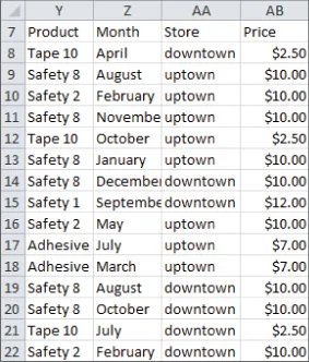
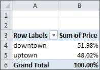
• What percentage of sales occurs at each store?
• What percentage of sales occurs during each month?
• How much revenue does each product generate?
• Which products generate 80 percent of the revenue?

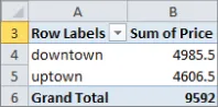
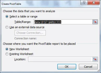
Calculating the Percentage of Sales at Each Store

The first step in creating a PivotTable is ensuring you have headings in the first row of your data. Notice that Row 7 of the example data in the data worksheet has the headings Product, Month, Store, and Price. Because these are in place, you can begin creating your PivotTable. To do so, perform the following steps:

1. Place your cursor anywhere in the data cells on the data worksheet, and then click PivotTable in the Tables group on the Insert tab. Excel opens the Create PivotTable dialog box, as shown in Figure 1.2, and correctly guesses that the data is included in the range Y7:AB1333.

Figure 1-2: PivotTable Dialog Box

---

NOTE

If you select Use an External Data Source here, you could also refer to a database as a source for a PivotTable. In Exercise 14 at the end of the chapter you can practice creating PivotTables from data in different worksheets or even different workbooks.

---

2. Click OK and you see the PivotTable Field List, as shown in Figure 1.3.

Figure 1-3: PivotTable Field List

3. Fill in the PivotTable Field List by dragging the PivotTable headings or fields into the boxes or zones. You can choose from the following four zones:

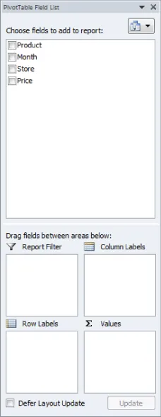
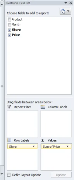
• Row Labels: Fields dragged here are listed on the left side of the table in the order in which they are added to the box. In the current example, the Store field should be dragged to the Row Labels box so that data can be summarized by store.
• Column Labels: Fields dragged here have their values listed across the top row of the PivotTable. In the current example no fields exist in the Column Labels zone.
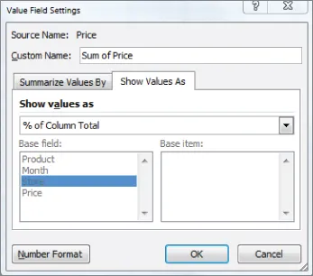
• Values: Fields dragged here are summarized mathematically in the PivotTable. The Price field should be dragged to this zone. Excel tries to guess the type of calculation you want to perform on a field. In this example Excel guesses that you want all Prices to be summed. Because you want to compute total revenue, this is correct. If you want to change the method of calculation for a data field to an average, a count, or something else, simply double-click the data field or choose Value Field Settings. You learn how to use the Value Fields Setting command later in this section.
• Report Filter: Beginning in Excel 2007, Report Filter is the new name for the Page Field area. For fields dragged to the Report Filter zone, you can easily pick any subset of the field values so that the PivotTable shows calculations based only on that subset. In Excel 2010 or Excel 2013 you can use the exciting Slicers to select the subset of fields used in PivotTable calculations. The use of the Report Filter and Slicers is shown in the “Report Filter and Slicers” section of this chapter.

---

NOTE

To see the field list, you need to be in a field in the PivotTable. If you do not see the field list, right-click any cell in the PivotTable, and select Show Field List.

---

Figure 1.4 shows the completed PivotTable Field List and the resulting PivotTable is shown in Figure 1.5 as well as on the FirstorePT worksheet.

Figure 1-4: Completed PivotTable Field List

Figure 1-5: Completed PivotTable

Figure 1.5 shows the downtown store sold $4,985.50 worth of goods, and the uptown store sold $4,606.50 of goods. The total sales are $9592.

If you want a percentage breakdown of the sales by store, you need to change the way Excel displays data in the Values zone. To do this, perform these steps:

1. Right-click in the summarized data in the FirstStorePT worksheet and select Value Field Settings.

2. Select Show Values As and click the drop-down arrow on the right side of the dialog box.

3. Select the % of Column Total option, as shown in Figure 1.6.

Figure 1-6: Obtaining percentage breakdown by Store

Figure 1.7 shows the resulting PivotTable with the new percentage breakdown by Store with 52 percent of the sales in the downtown store and 48 percent in the uptown store. You can also see this in the revenue by store worksheet of the PARETO.xlsx file.

Figure 1-7: Percentage breakdown by Store

---

NOTE

If you want a PivotTable to incorporate a different set of data, then under Options, you can select Change Data Source and select the new source data. To have a PivotTable incorporate changes in the original source data, simply right-click and select Refresh. If you are going to add new data below the original data and you want the PivotTable to include the new data...