Proportionate-type Normalized Least Mean Square Algorithms

Kevin Wagner, Milos Doroslovacki

• Publisher: Wiley-ISTE
• Year: 2013
• ISBN:
  9781118579251
• Edition: 1
• Topic: Ciencia de la computación
• Subtopic: Algoritmos de programación

The topic of this book is proportionate-type normalized least mean squares (PtNLMS) adaptive filtering algorithms, which attempt to estimate an unknown impulse response by adaptively giving gains proportionate to an estimate of the impulse response and the current measured error. These algorithms offer low computational complexity and fast convergence times for sparse impulse responses in network and acoustic echo cancellation applications. New PtNLMS algorithms are developed by choosing gains that optimize user-defined criteria, such as mean square error, at all times. PtNLMS algorithms are extended from real-valued signals to complex-valued signals. The computational complexity of the presented algorithms is examined.

Contents

1. Introduction to PtNLMS Algorithms
2. LMS Analysis Techniques
3. PtNLMS Analysis Techniques
4. Algorithms Designed Based on Minimization of User Defined Criteria
5. Probability Density of WD for PtLMS Algorithms
6. Adaptive Step-size PtNLMS Algorithms
7. Complex PtNLMS Algorithms
8. Computational Complexity for PtNLMS Algorithms

About the Authors

Kevin Wagner has been a physicist with the Radar Division of the Naval Research Laboratory, Washington, DC, USA since 2001. His research interests are in the area of adaptive signal processing and non-convex optimization.
Milos Doroslovacki has been with the Department of Electrical and Computer Engineering at George Washington University, USA since 1995, where he is now an Associate Professor. His main research interests are in the fields of adaptive signal processing, communication signals and systems, discrete-time signal and system theory, and wavelets and their applications.

1

Introduction to PtNLMS Algorithms

The objective of this chapter is to introduce proportionate-type normalized least mean square (PtNLMS) algorithms in preparation for performing analysis of these algorithms in subsequent chapters. In section 1.1, we begin by presenting applications for PtNLMS algorithms as the motivation for why analysis and design of PtNLMS algorithms is a worthwhile cause. In section 1.2, a historical review of relevant algorithms and literature is given. This review is by no means exhaustive; however, it should serve the needs of this work by acting as a foundation for the analysis that follows. In section 1.3, standard notation and a unified framework for representing PtNLMS algorithms are presented. This notation and framework will be used throughout the remainder of this book. Finally, with this standardized notation and framework in hand, we present several PtNLMS algorithms in section 1.4. The chosen PtNLMS algorithms will be referenced frequently throughout this work.

1.1. Applications motivating PtNLMS algorithms

Historically, PtNLMS algorithms have found use in network echo cancellation applications as a method for reducing the presence of delayed copies of the original signal, i.e. echoes. For instance, in many telephone communication systems the network consists of two types of wire segments: a four-wire central network and a two-wire local network [MIN 06]. A converting device, called a hybrid, is needed at the junction of the two-wire to four-wire segments. When a far-end user talks a portion of the signal is reflected back to the far-end listener, due to the impedance mismatch in the hybrid as shown in Figure 1.1. This type of echo is called electric echo or circuit echo. An adaptive filter can be used to estimate the impulse response of the hybrid and remove the echo caused by the hybrid.

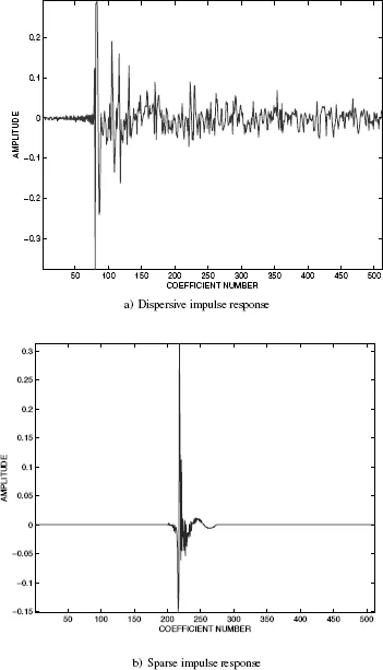
In modern telephone networks, greater delays increase the need for echo cancellation. Specifically, these communication networks have driven the need for faster converging echo cancellation algorithms when the echo path is sparse. A sparse echo path is that in which a large percentage of the energy is distributed to only a few coefficients. Conversely, a dispersive echo path has distributed most of its energy more or less evenly across all of the coefficients. Examples of a dispersive impulse response and a sparse impulse response are shown in Figures 1.2a and 1.2b, respectively. While most network echo path cancelers have echo path lengths in the order of 64 ms, the active part of the echo path is usually only about 4–6 ms long [GAY 98], hence the echo path is sparse. The active part of an echo path corresponds to the coefficients of the echo path that contain the majority of the energy. When the impulse response is sparse, PtNLMS algorithms can offer improved performance relative to standard algorithms such as the least mean square (LMS) and normalized least mean square (NLMS) [HAY 02].

Figure 1.1. Telephone echo example

Another application for PtNLMS has been spawned by the emergence of Voice over IP (VOIP) as an important and viable alternative to circuit switched networks. In these systems, longer delays are introduced due to packetization [SON 06]. In addition, echoes can be created during the transition from traditional telephone circuits to IP-based telephone networks [MIN 06].

The advent of telephone communication via satellite has motivated the search for a better way to eliminate echoes [WEI 77]. The distortion caused by echo suppressors is particularly noticeable on satellite-routed connections.

Let us also mention that modern applications of echo cancellation include acoustic underwater communication where the impulse response is often sparse [STO 09], television signals where the delay can be significant due to satellite communication [SCH 95], high-definition television terrestrial transmission that requires equalization due to inter-symbol interference caused by multi-path channels exhibiting sparse behavior [FAN 05], and applications where the impulse response is sparse in the transform domain [DEN 07].

Figure 1.2. Dispersive and sparse impulse responses

When examining these applications as well as others like them, several questions regarding the desired performance of the PtNLMS algorithms need to be answered in order to design an algorithm for the intended application. For instance, we need to know what the required convergence of the algorithm needs to be. We also need to know the computational complexity that the application can support as well as what level of steady-state bias can be tolerated. To address these questions we need to understand the underlying mechanics of each PtNLMS algorithm as well as what factors control how the algorithms perform. Therefore, we intend to analyze PtNLMS algorithms to find out what factors influence the convergence, steady-state performance, and what the implementation cost of possible improvements in terms of computational complexity is. In doing so, a better understanding of what influences the performance of PtNLMS algorithms is provided. Answering these questions will allow us to design algorithms that perform their desired tasks more efficiently.

1.2. Historical review of existing PtNLMS algorithms

In the past, adaptive filtering algorithms such as the LMS and NLMS have been examined extensively [HAY 02]. These algorithms offer low computational complexity and proven robustness. The LMS and NLMS algorithms share the property of the adaptive weights being updated in the direction of the input vector. These algorithms perform favorably in most adaptive filtering situations.

The LMS and NLMS algorithms fall within the larger class of PtNLMS algorithms. PtNLMS algorithms can update the adaptive filter coefficients such that some coefficients are favored. That is, some coefficients receive more emphasis during the update process. Because of this fact, the PtNLMS algorithms are better suited to deal with sparse impulse responses.

An example of a PtNLMS algorithm is the proportionate normalized least mean square (PNLMS) algorithm [DUT 00]. This algorithm updates the adaptive filter coefficients by assigning a gain proportional to the magnitude of the current coefficient estimates. This approach improves the initial convergence rates. However, this gain adaptation scheme causes the PNLMS algorithm to suffer from slow convergence of small coefficients, and as a result the time needed to reach steady-state error is increased compared to the NLMS algorithm. The PNLMS algorithm has been shown to outperform the LMS and NLMS algorithms when operating on a sparse impulse response. Currently, any analytical model to describe learning curve convergence of the PNLMS algorithm does not exist [SON 06].

Another weakness of the PNLMS algorithm is that when the impulse response is dispersive, the algorithm converges much slower than the NLMS algorithm. To remedy this issue the PNLMS++ was proposed [GAY 98]. The PNLMS++ algorithm solves this issue by alternating between the NLMS and PNLMS algorithms on each sample period of the algorithm. The improved PNLMS (IPNLMS) was introduced to build upon the PNLMS++ algorithm [BEN 02]. The IPNLMS attempts to exploit the shape of the estimated echo, instead of blindly alternating between the PNLMS and NLMS algorithms as is done in the PNLMS++ algorithm. The IPNLMS algorithm performs better than the NLMS and PNLMS algorithms no matter what the nature of the impulse response.

In the following, the improved IPNLMS (IIPNLMS) algorithm was proposed [CUI 04]. This algorithm attempted to identify active and inactive regions of the echo path impulse response. Active regions received updates more in-line with the NLMS methodology, while inactive regions received gains based upon the PNLMS methodology. In this way, the IIPNLMS was able to outperform the IPNLMS algorithm. The idea of applying gain selectively to active and inactive regions was explored previously in the so-called partial update algorithms. These algorithms, motivated by reducing computational complexity while improving performance, update a subset of all the coefficients during each sampling period. Examples of partial update NLMS algorithms can be found in [TAN 02] and [NAY 03].

Another set of algorithms was designed by seeking a condition to achieve the fastest overall convergence. Initially, the steepest descent algorithm was optimized and then the resulting deterministic algorithm was cast into the stochastic framework. It can be shown that the total number of iterations for overall convergence is minimized when all of the coefficients reach the ∊-vicinity of their true values simultaneously (where ∊ is some small positive number). This approach results in the μ-law PNLMS (MPNLMS) [DEN 05]. The MPNLMS algorithm addresses the issue of assigning too much update gain to large coefficients, which occurs in the PNLMS algorithms.

The ∊-law PNLMS (EPNLMS) [WAG 06] algorithm is a second implementation of the same philosophy used to generate the MPNLMS algorithm. This algorithm gives the minimum gain possible to all of the coefficients with magnitude less than ∊. It assumes that the impulse response is sparse and contains many small magnitude coefficien...