Volatility Trading

Euan Sinclair

• Publisher: Wiley
• Year: 2013
• ISBN:
  9781118416723
• Edition: 1
• Topic: Business
• Subtopic: Finance
• Index: Business

Popular guide to options pricing and position sizing for quant traders

In this second edition of this bestselling book, Sinclair offers a quantitative model for measuring volatility in order to gain an edge in everyday option trading endeavors. With an accessible, straightforward approach, he guides traders through the basics of option pricing, volatility measurement, hedging, money management, and trade evaluation. This new edition includes new chapters on the dynamics of realized and implied volatilities, trading the variance premium and using options to trade special situations in equity markets.

• Filled with volatility models including brand new option trades for quant traders
• Options trader Euan Sinclair specializes in the design and implementation of quantitative trading strategies

Volatility Trading, Second Edition + Website outlines strategies for defining a true edge in the market using options to trade volatility profitably.

Chapter 1

Option Pricing

It is possible to trade options without any valuation model. For example, traders might buy a call option because they think the underlying will rally further past the strike than the price they have paid. This is the simplest, most direct use of options. At a level of complexity only slightly greater than this we can trade volatility without a model. Traders might sell a straddle because they think the underlying will expire closer to the strike than the value of the straddle. There are an enormous number of option positions like this where traders can attempt to profit from their opinion of the future distribution of the underlying. However, if we want to express an opinion based on the behavior of the underlying before expiration, we will need a model.

A model is a framework we can use to compare options of different maturities, underlyings, and strikes. We do not insist that it is in any sense true or even a particularly accurate reflection of the real world. As options are highly leveraged, nonlinear, time-dependent bets on the underlying their prices change quickly. The major goal of a pricing model is to translate these prices into a more slowly moving system.

A model that perfectly captures all aspects of a financial market is probably unobtainable. Further, even if it existed it would be too complex to calibrate and use. So we need to somewhat simplify the world in order to model it. Still, with any model we must be aware of the simplifying assumptions that are being used and the range of applicability.

The Black-Scholes-Merton Model

We will present an analysis of the Black-Scholes-Merton (BSM) equation. The BSM formalism becomes the conceptual framework for an options trader: In the same way that we hear our thoughts in English, an experienced derivatives trader thinks in the BSM language. This is an important difference between the models used by traders and the models used in a hard science such as physics. Models in physics aim to make statements about the world that are at least in some sense true, and then use the model to make predictions. The degree of truth needn't be consistent between all models. There are some successful theories that are based on highly simplified phenomenological models. An example would be Rutherford's model of the atom, which assumes that electrons orbit the nucleus like planets orbit the sun. This contains some truth: The atom consists of electrons and nuclear particles, but the planetary model isn't an accurate depiction of atomic structure.

Trading models are fundamentally different. The BSM model isn't good because it is an accurate representation of reality. It is actually fairly poor in this regard, with most of the model's assumptions being gross oversimplifications. It is a good model because the weaknesses are well understood and the model gives results that are intuitively sensible. The model fits its purpose. It is useful. It makes as little sense to say it is correct or incorrect as to say that German is incorrect and French is correct.

The standard derivation of the BSM equation can be found in any number of places (for example, Hull 2005). Although good derivations carefully lead us through the mathematics and financial assumptions they don't generally make it obvious what to do as a trader. We must always remember that our goal is to identify and profit from mispriced options. How does the BSM formalism help us do this?

Here we approach the problem backward. We start from the assumption that a trader holds a delta-hedged portfolio consisting of a call option and Δ units of short stock. We then apply our knowledge of option dynamics to derive the BSM equation.

That this portfolio is delta hedged should be obvious to option traders. Actually, traders knew about delta hedging long before BSM (for an interesting history, refer to Haug 2007a). But even if this is the first derivation of BSM the reader has seen this shouldn't be a remarkable fact. A call (put) option gains (declines) in value as the underlying rises. So in principle we can offset this directional risk with a position in the underlying. This should be obvious. The details of exactly how much of the underlying to hold are certainly not obvious.

Even before we make any assumptions about the distribution of the underlying's returns, we can state a number of the properties that an option must possess. These should be financially obvious.

• A call (put) becomes more valuable as the underlying rises (falls), as it has more chance of becoming intrinsically valuable.
• The value of a call (put) can never be more than the value of the underlying (strike).
• An option loses value as time passes, as it has less time to become intrinsically valuable.
• An option must have positive dependence on uncertainty. If the underlying had no risk there would be no need to pay for a product that only has value in certain states of the world. Options only have value because we are uncertain about the future, so it follows that the more uncertain we are the more valuable the options will be.
• An option loses value as rates increase. Because we have to borrow money to pay for options, as rates increase our financing costs increase, ignoring for now any rate effects on the underlying.
• Dividends (and storage or borrowing costs) have different effects on calls and puts. The holder of an option does not receive the dividend. This means that a dividend lowers the effective value of the underlying stock for the purposes of option valuation. So a dividend increases the value of a put and lowers the value of a call.

As we have said, even before the invention of the BSM formalism, option traders were aware that directional risk could be mitigated by combining their options with a position in the underlying. So let's assume we hold the delta-hedged option position,

1.1

where C is the value of the option, S_t is the underlying price at time, t, and Δ is the number of shares we are short. Over the next time step the underlying changes to S_t+1. The change in the value of the portfolio is given by the change in the option and stock positions together with any financing charges we incur by borrowing money to pay for the position.

1.2

To see why the last term is positive we need to consider our cash flows. We bought the option, so we need to finance that cost, but we shorted stock so we receive money for this. Over a single time step we gain rΔS_t from this.

Note also that we assume that the time step is small enough that we can take delta to be unchanged.

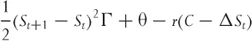
The change in the option value due to the underlying price change can be approximated by a second-order Taylor expansion. Also we know that when “other things are held constant,” the option will decrease due to the passing of time by an amount denoted by θ.

At this point in our argument we have assumed that we need to consider second derivatives with respect to price but only first derivatives with respect to time. Why is either of these choices valid? Ignoring higher derivatives with respect to price really cannot be justified at this point. We have only done it because we are trying to recover the BSM equation. In a more formal derivation this would be related to the assumption of a normal distribution of underlying returns. This is a major simplification that I am not ignoring. I'm postponing the discussion until later. The assumption that we need fewer derivatives with respect to time is easier to justify. Underlying price changes are stochastic and so they are a source of risk. Time change is predictable and the effect of time on options is merely a cost.

So we get

1.3

or

1.4

where Γ is the second derivative of the option price with respect to the underlying. Equation 1.4 gives the change in value of the portfolio, or the profit the trader makes when the stock price changes by a small amount. It has three separate components.

1. The first term gives the effect of gamma. Since gamma is positive, the option holder makes money. The return is proportional to half the square of the underlying price change.

2. The second term gives the effect of theta. The option holder loses money due to the passing of time.

3. The third term gives the effect of financing. Holding a hedged long option portfolio is equivalent to lending money.

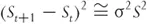
Further, we see in the next chapter that on average

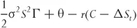
where σ is the standard deviation of the underlying's returns, generally known as volatility. So we can rewrite Equation 1.4 as

1.5

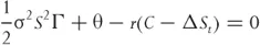
If we accept that this position should not earn any abnormal profits because it is riskless and financed with borrowed money, the equation can be set equal to zero. Therefore, the equation for the fair value of the option is

1.6

Before continuing, we need to make explicit some of the assumptions that this informal derivation has hidden.

• To write down Equation 1.1, we needed to assume the existence of a tradable underlying asset. In fact we assumed that it could be shorted and the underlying could be traded in any size necessary without incurring transaction costs.
• Equation 1.2 has assumed that the proceeds from the short sale can be reinvested at the same interest rate at which we have borrowed to finance the purchase of the call. We have also ta...