Volatility Trading

Euan Sinclair

• Publisher: Wiley
• Year: 2011
• ISBN:
  9781118045299
• Edition: 1
• Topic: Business
• Subtopic: Finance
• Index: Business

In Volatility Trading, Sinclair offers you a quantitative model for measuring volatility in order to gain an edge in your everyday option trading endeavors. With an accessible, straightforward approach. He guides traders through the basics of option pricing, volatility measurement, hedging, money management, and trade evaluation. In addition, Sinclair explains the often-overlooked psychological aspects of trading, revealing both how behavioral psychology can create market conditions traders can take advantage of-and how it can lead them astray. Psychological biases, he asserts, are probably the drivers behind most sources of edge available to a volatility trader. Your goal, Sinclair explains, must be clearly defined and easily expressed-if you cannot explain it in one sentence, you probably aren't completely clear about what it is. The same applies to your statistical edge. If you do not know exactly what your edge is, you shouldn't trade. He shows how, in addition to the numerical evaluation of a potential trade, you should be able to identify and evaluate the reason why implied volatility is priced where it is, that is, why an edge exists. This means it is also necessary to be on top of recent news stories, sector trends, and behavioral psychology. Finally, Sinclair underscores why trades need to be sized correctly, which means that each trade is evaluated according to its projected return and risk in the overall context of your goals. As the author concludes, while we also need to pay attention to seemingly mundane things like having good execution software, a comfortable office, and getting enough sleep, it is knowledge that is the ultimate source of edge. So, all else being equal, the trader with the greater knowledge will be the more successful. This book, and its companion CD-ROM, will provide that knowledge. The CD-ROM includes spreadsheets designed to help you forecast volatility and evaluate trades together with simulation engines.

CHAPTER 1

Option Pricing

In order to profitably trade options we need a model for valuing them. This is a framework we can use to compare options of different maturities, underlyings, and strikes. We do not insist that it is in any sense true or even a particularly accurate reflection of the real world. As options are highly leveraged, nonlinear, time-dependent bets on the underlying, their prices change very quickly. The major goal of a pricing model is to translate these prices into a more slowly moving system.

A model that perfectly captures all aspects of a financial market is probably unobtainable. Further, even if it existed it would be too complex to calibrate and use. So we need to somewhat simplify the world in order to model it. Still, with any model we must be aware of the simplifying assumptions that are being used and the range of applicability. The specific choice of model isn’t as important as developing this level of understanding.

THE BLACK-SCHOLES-MERTON MODEL

We present here an analysis of the Black-Scholes-Merton (BSM) equation. The BSM formalism becomes the conceptual framework for an options trader: In the same way that we hear our own thoughts in English, an experienced derivatives trader thinks in the BSM language.

The standard derivation of the BSM equation can be found in any number of places (for example, Hull 2005). While good derivations carefully lead us through the mathematics and financial assumptions, they don’t generally make it obvious what to do as a trader. We must always remember that our goal is to identify and profit from mispriced options. How does the BSM formalism help us do this?

Here we approach the problem backwards. We start from the assumption that a trader holds a delta hedged portfolio consisting of a call option and Δ units of short stock.² We then apply our knowledge of option dynamics to derive the BSM equation.

Even before we make any assumptions about the distribution of underlying returns, we can state a number of the properties that an option must possess. These should be financially obvious.

• A call (put) becomes more valuable as the underlying rises (falls), as it has more chance of becoming intrinsically valuable.

• An option loses value as time passes, as it has less time to become intrinsically valuable.

• An option loses value as rates increase. Since we have to borrow money to pay for options, as rates increase our financing costs increase, ignoring for now any rate effects on the underlying.

• The value of a call (put) can never be more than the value of the underlying (strike).

As we have said, even before the invention of the BSM formalism, option traders were aware that directional risk could be mitigated by combining their options with a position in the underlying. So let’s assume we hold the delta hedged option position,

(1.1)

where

C is the value of the option
S_t is the underlying price at time t
Δ is the number of shares we are short

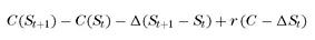
Over the next time step the underlying changes to S_t+1. The change in the value of the portfolio is given by the change in the option and stock positions together with any financing charges we incur by borrowing money to pay for the position.

(1.2)

The last term is written as positive because we know that the value of the long call/short stock portfolio will be negative (or at most zero when Δ is 1) and hence will have us lending money and thus receiving interest income. Note also that we assume the time step is small enough that we can take delta to be unchanged.

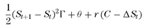
The change in the option value due to the underlying price change can be approximated by a second-order Taylor expansion. Also, we know that when other things are held constant, the option will decrease due to the passing of time by an amount denoted by θ.

So we get

(1.3)

Or

(1.4)

where Γ is the second derivative of the option price with respect to the underlying.

Expression (1.4) gives the change in value of the portfolio, or the profit the trader makes when the stock price changes by a small amount. It has three separate components:

1. The first term gives the effect of gamma. Since gamma is positive, the option holder makes money. The return is proportional to half the square of the underlying price change.

2. The second term gives the effect of theta. The option holder loses money due to the passing of time.

3. The third term gives the effect of financing. Holding a hedged long option portfolio is equivalent to lending money.

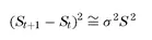
Further, we see in Chapter 2 that on average

where σ is the standard deviation of the underlying’s returns, generally known as volatility.

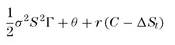
So we can rewrite expression (1.4) as

(1.5)

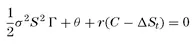
If we accept that this position should not earn any abnormal profits because it is riskless and financed with borrowed money, the expression can be set equal to zero. Therefore the equation for the fair value of the option is

(1.6)

Before continuing, we need to make explicit some of the assumptions that this informal derivation has hidden.

• In order to write down expression (1.1) we needed to assume the existence of a tradable underlying asset. In fact, we assume that it can be shorted and the underlying can be traded in any size necessary without incurring transaction costs.

• Expression (1.2) has assumed that the proceeds from the short sale can be reinvested at the same interest rate at which we have borrowed to finance the purchase of the call. We have also taken this rate to be constant.

• Expression (1.3) has assumed that the underlying changes are continuous and smooth. Further, we have considered second-order derivatives with respect to price but only first-order with respect to time.

But something about which we haven’t made any assumptions at all is whether the underlying has any drift. This is remarkable. We may naively assume that an instrument whose value increases as the underlying asset rises would be dependent on its drift. However, the effect of drift can be negated by combining the option with the share in the correct proportion. As the drift can be hedged away, the holder of the option is not compensated for it. When we consider hedging later in Chapter 4, we find that in the real world, where the assumptions about continuity fail, directional dependence will reemerge.

However, note that while the price change does not appear in equation (1.6), the square of the price change does through the volatility term. So the magnitude of the price changes is central to whether the trader makes a profit with a delta hedged position. This is true whether or not returns are normally distributed. As long as the variance of returns is finite, this result holds. In fact, if we had included higher-order price terms in the Taylor expansion, we would see that the option’s price change also depended on higher-order price differences.

With appropriate final conditions, equation (1.6) holds for a variety of instruments: European and American options, calls and puts, and many exotics. It can be solved with any of the usual methods for solving partial differential equations.

In this exercise we have derived a form of the BSM equation by working backwards from our trader’s knowledge of how options react to changes in underlying and time. In doing so, it has given us what we need to know to trade options from the point of volatility.

We have shown how the fair price for an option is related to the standard deviation of the underlying returns. Since at any time there is an option market and the underlying market, there are two ways we can proceed:

1. Using the quoted price of the option, calculate the implied standard deviation or volatility.

2. Using an estimate of the volatility over the life of the option, calculate a theoretical option price.

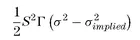
If our estimate of volatility differs significantly from that implied by the option market, then we can trade the option accordingly. If we forecast volatility to be higher than that implied by the option, we would buy the option and hedge in the underlying market. Our expected profit would depend on the difference between implied volatility and realized volatility. Equation (1.6) says that instantaneously this profit would be proportional to

(1.7)

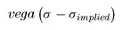
A complementary way to think of the expected profit of a hedged option is by considering vega. Vega is defined as the change in value of an option if implied volatility changes by one point (e.g., from 19 to 18 percent). This means that if we buy an option at σ_implied and volatility immediately increases to σ we would make a profit of

(1.8)

If we have to hold the option to expiration and realized volatility averages σ we will also make this amount, but only on average. The vega profit is realized as the sum of the hedges as we rebalance our delta. This can be formalized by noting the relationship between vega and gamma,

(1.9)

So expression (1.7) can also be written as

(1.10)

The problem this presents is that the gamma is highly dependent on the moneyness of the option, which obviously ...