Machine Learning in Python

Hands on Machine Learning with Python Tools, Concepts and Techniques

Bob Mather

• Publisher: Abiprod
• Year: 2019
• ISBN:
  9781922300034
• Topic: Ciencia de la computación
• Subtopic: Inteligencia artificial (IA) y semántica

Are you excited about Artificial Intelligence and want to get started?Are you excited about Machine Learning and want to learn how to implement in Python?

The book below is the answer. Given the large amounts of data we use everyday; whether it is in the web, supermarkets, social media etc. analysis of data has become integral to our daily life. The ability to do so effectively can propel your career or business to great heights. Machine Learning is the most effective data analysis tool. While it is a complex topic, it can be broken down into simpler steps, as show in this book. We are using Python, which is a great programming language for beginners. Python is a great language that is commonly used with Machine Learning. Python is used extensively in Mathematics, Gaming and Graphic Design. It is fast to develop and prototype. It is web capable, meaning that we can use Python to gather web data. It is adaptable, and has great community of users.

Here's What's Included In This Book:

What is Machine Learning?Why use Python?Regression Analysis using Python with an exampleClustering Analysis using Python with an exampleImplementing an Artificial Neural NetworkBackpropagation90 Day Plan to Learn and Implement Machine LearningConclusion

Regression Analysis using Python

What is Regression Analysis?

Now, if you recall, I actually started this book off by comparing the y-intercept formula and Regression Analysis actually utilizes an equation very similar to this.

In this equation, we are saying that the y is equal to that of the y-intercept population parameter plus the slope population parameter plus the error term. The error term is labeled as such because it represents for the unexplained variation in the equation for solving y. Essentially, this is the part of the equation we’re ultimately trying to reduce so that we can have accurate results. Ultimately, the ideal equation is found below:

The expected y, which can also be donated as

when working with sample data, is equal to that of the sum of the y-intercept population and slope population parameters. Now, let’s back up here because you might not actually understand how to calculate the error term in this equation when you first start out.

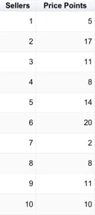
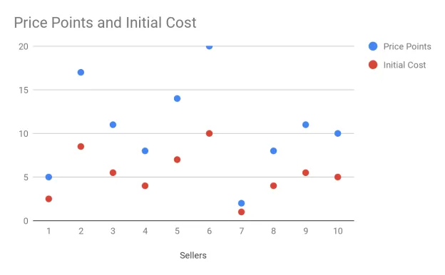
Alright, so let’s start out by going to the market to negotiate how many trinkets we can buy and for how much. There is no set price for the trinkets and we are buying the same trinket from different sellers. Here is a table that lists 10 sellers and their different price points for selling their trinket to us.

In this table, we can see that we have a price point for each of them. Now, can you predict what the next price point will be for the 11th seller in such a graph? Since the only definition we have right now is the price point, the best next prediction will be the mean. The mean is the amount at which there is a 50/50 expectation that it will be the correct prediction. To calculate the mean, we simply add up all the price points and divide them by the number of price points that there are. The mean for this table is 10.6.

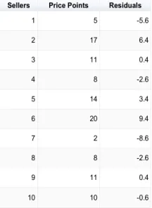
Now that we have out mean value, we can now calculate for our residuals. A residual is a number that deviates from the mean value. While technically all of the values deviate from this, the residual is how much it deviates from the mean. Thus, here is our new table.

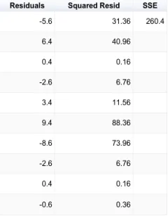
Something to keep in mind here is that the Residuals are the actual Errors we are talking about in Regression Analysis. Now we need to find the Sum of Squared Errors or the Sum of Squared Residuals. In the following table, I have done just that.

Now, you might be wondering why we are going through these very specific steps. Simple Linear Regression, the most basic form of Regression Analysis, is based on reducing the SSE (Sum of Squared Errors) to create a Best Fit Line. In Linear Regression, we are comparing this SSE that we got when we assumed there was only 1-set of categorizing data (the dependent variable) to another that has 2 sets of categorizing data (the independent and dependent variable). Linear Regression is a part of a special type of mathematics known as Bivariate Statistics. Bivariate means that there are two variables or variations in the Statistics that you may be studying.

In Linear Regression, the Y-Axis is meant to be the “Why?” while the X-Axis is meant to be the “Explanation” of the data. Therefore, “Why is price point 1 at 5?” and then our X-Axis would be used to explain why it is there. You may have also seen that I included a slope in a previous table and that is because the data does have a slope. However, when you are using an equation like this:

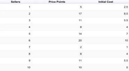
Where the sample data expected y is equal to that of the sample data y-intercept population plus the slope population in order to calculate for 1 variable, you are using a slope of zero. Now we’re going to go ahead and add a 2nd variable to our equation, which will be how much money it costs the seller to actually buy the trinket from the person who made it. We will call this new variable the Initial Cost as it is the initial cost of the trinket before it is marked up for profit by other sellers. The Price Point is DEPENDENT on the Initial Cost, which a very important distinction to make. Remember that I said that the Y-Axis is the why, thus the Price Point is our new Y plot point and the Initial Cost is our X plot point. Now, here comes a new equation:

This is known as the Least Squares equation. If you remember correctly, the hat of y is the result we get from our sample data where our Initial Cost didn’t exist. The reason why the second y in this equation does not have a hat is because this y is what we will observe of the actual data. The hat of y is our predicted data while the regular y is that actual data. We will be finding the difference of these two, but not on a graph by graph basis. This equation requires us to minimize the sum of the squared differences of each predicted y with each observed y in a linear progression. Here is the new data we will be utilizing:

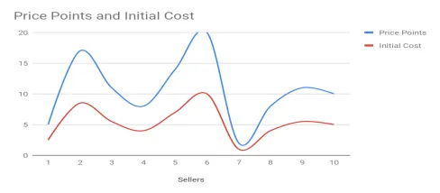
I am aware of how clear cut this is, but this is because we’re utilizing fake data to make this easier to understand. In the real world, you could spend weeks only to find there’s no correlation so for teaching purposes it is much better to have a mock scenario. Instead of looking at this data, you would be putting it in a Scatter Plot like this:

In this graph, it is not as clear that there is a correlation, and this is why data representation is key to seeing the relation between the two. For instance, if I ran this in a Line Graph, the correlation would be glaring:

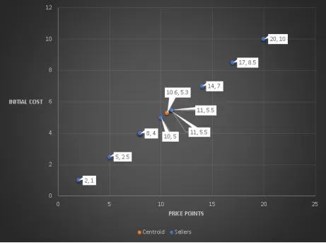
The next step in this process is to find what is known as the Centroid and it represents the point at which our Regression Best Fit Line will pass through.

As you can already tell, our Regression Line will most likely go straight through that line. So, the first step in plotting this Regression Line is to find the Slope or the

of our equation and that equation requires a bigger equation:

Now, this could very well look rather scary at first, but this equation is actually quite simple. On top, we are finding the difference between the independent (initial cost) variable as x and the mean of that independent variable as well as between the dependent variable as y and the mean of the dependent variable. Then we multiply those together. Once we are all done doing these to all of the variables, we then add all of those results together before dividing. On the bottom of our division, we take the independent variable and subtract the mean of the independent variable, but then we square that result. Once we do this to all of them, we add all the results together. Here it is in Python. I prefer to view math in code quite often rather than the equation:

independent_var = [2.5,8.5,5.5,4,7,10,1,4,5.5,5] independent_mean = 5.3 dependent_var = [5,17,11,8,14,20,2,8,11,10] dependent_mean = 10.6 def slope(independent_var, independent_mean, dependent_var, dependent_mean): d = [] x = [] top = 0 y = 0 for i in range(len(independent_var)): x.append(independent_var[i] - independent_mean) for i in range(len(dependent_var)): d.append(dependent_var[i] - dependent_mean) for i in range(len(x)): top += x[i] * d[i] for i in range(len(independent_var)): y += (independent_var[i] - independent_mean)**2 print(top/y) return top/y pass

As you can see, it’s relatively basic in what needs to be done but you now need to feed it into the other side of the equation.

The answer to our slope was 2. This will now be multiplied against the independent mean (x bar) and subtracted from the dependent mean (y bar) to equal

. In our case, using the modified algorithm:

independent_var = [2.5,8....