R Deep Learning Essentials

A step-by-step guide to building deep learning models using TensorFlow, Keras, and MXNet, 2nd Edition

Mark Hodnett, Joshua F. Wiley

• Publisher: Packt Publishing
• Year: 2018
• ISBN:
  9781788997805
• Edition: 2
• Topic: Informatica
• Subtopic: Elaborazione del linguaggio naturale

Implement neural network models in R 3.5 using TensorFlow, Keras, and MXNet

Key Features

• Use R 3.5 for building deep learning models for computer vision and text
• Apply deep learning techniques in cloud for large-scale processing
• Build, train, and optimize neural network models on a range of datasets

Book Description

Deep learning is a powerful subset of machine learning that is very successful in domains such as computer vision and natural language processing (NLP). This second edition of R Deep Learning Essentials will open the gates for you to enter the world of neural networks by building powerful deep learning models using the R ecosystem.

This book will introduce you to the basic principles of deep learning and teach you to build a neural network model from scratch. As you make your way through the book, you will explore deep learning libraries, such as Keras, MXNet, and TensorFlow, and create interesting deep learning models for a variety of tasks and problems, including structured data, computer vision, text data, anomaly detection, and recommendation systems. You'll cover advanced topics, such as generative adversarial networks (GANs), transfer learning, and large-scale deep learning in the cloud. In the concluding chapters, you will learn about the theoretical concepts of deep learning projects, such as model optimization, overfitting, and data augmentation, together with other advanced topics.

By the end of this book, you will be fully prepared and able to implement deep learning concepts in your research work or projects.

What you will learn

• Build shallow neural network prediction models
• Prevent models from overfitting the data to improve generalizability
• Explore techniques for finding the best hyperparameters for deep learning models
• Create NLP models using Keras and TensorFlow in R
• Use deep learning for computer vision tasks
• Implement deep learning tasks, such as NLP, recommendation systems, and autoencoders

Who this book is for

This second edition of R Deep Learning Essentials is for aspiring data scientists, data analysts, machine learning developers, and deep learning enthusiasts who are well versed in machine learning concepts and are looking to explore the deep learning paradigm using R. Fundamental understanding of the R language is necessary to get the most out of this book.

Training Deep Prediction Models

The previous chapters covered a bit of the theory behind neural networks and used some neural network packages in R. Now it is time to dive in and look at training deep learning models. In this chapter, we will explore how to train and build feedforward neural networks, which are the most common type of deep learning model. We will use MXNet to build deep learning models to perform classification and regression using a retail dataset.

This chapter will cover the following topics:

• Getting started with deep feedforward neural networks
• Common activation functions – rectifiers, hyperbolic tangent, and maxout
• Introduction to the MXNet deep learning library
• Use case – Using MXNet for classification and regression

Getting started with deep feedforward neural networks

A deep feedforward neural network is designed to approximate a function, f(), that maps some set of input variables, x, to an output variable, y. They are called feedforward neural networks because information flows from the input through each successive layer as far as the output, and there are no feedback or recursive loops (models including both forward and backward connections are referred to as recurrent neural networks).

Deep feedforward neural networks are applicable to a wide range of problems, and are particularly useful for applications such as image classification. More generally, feedforward neural networks are useful for prediction and classification where there is a clearly defined outcome (what digit an image contains, whether someone is walking upstairs or walking on a flat surface, the presence/absence of disease, and so on).

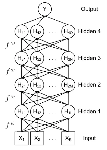
Deep feedforward neural networks can be constructed by chaining layers or functions together. For example, a network with four hidden layers is shown in the following diagram:

Figure 4.1: A deep feedforward neural network

This diagram of the model is a directed acyclic graph. Represented as a function, the overall mapping from the input, X, to the output, Y, is a multilayered function. The first hidden layer is H₁=f⁽¹⁾(X, w₁ a₁), the second hidden layer is H₂=f⁽²⁾(H₁, w₂ a₂), and so on. These multiple layers can allow complex functions and transformations to be built up from relatively simple ones.

If sufficient hidden neurons are included in a layer, it can approximate to the desired degree of precision with many different types of functions. Feedforward neural networks can approximate non-linear functions by applying non-linear transformations between layers. These non-linear functions are known as activation functions, which we will cover in the next section.

The weights for each layer will be learned as the model is trained through forward- and backward-propagation. Another key piece of the model that must be determined is the cost, or loss, function. The two most commonly used cost functions are cross-entropy, which is used for classification tasks, and mean squared error (MSE), which is used for regression tasks.

Activation functions

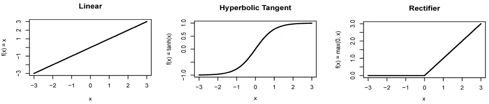
The activation function determines the mapping between input and a hidden layer. It defines the functional form for how a neuron gets activated. For example, a linear activation function could be defined as: f(x) = x, in which case the value for the neuron would be the raw input, x. A linear activation function is shown in the top panel of Figure 4.2. Linear activation functions are rarely used because in practice deep learning models would find it difficult to learn non-linear functional forms using linear activation functions. In previous chapters, we used the hyperbolic tangent as an activation function, namely f(x) = tanh(x). Hyperbolic tangent can work well in some cases, but a potential limitation is that at either low or high values, it saturates, as shown in the middle panel of the figure 4.2.

Perhaps the most popular activation function currently, and a good first choice (Nair, V., and Hinton, G. E. (2010)), is known as a rectifier. There are different kinds of rectifiers, but the most common is defined by the f(x) = max(0, x) function, which is known as relu. The relu activation is flat below zero and linear above zero; an example is shown in Figure 4.2.

The final type of activation function we will discuss is maxout (Goodfellow, Warde­-Farley, Mirza, Courville, and Bengio (2013)). A maxout unit takes the maximum value of its input, although as usual, this is after weighting so it is not the case that the input variable with the highest value will always win. Maxout activation functions seem to work particularly well with dropout.

The relu activation is the most commonly-used activation function and it is the default option for the deep learning models in the rest of this book. The following graphs for some of the activation functions we have discussed:

Figure 4.2: Common activation functions

Introduction to the MXNet deep learning library

The deep learning libraries we will use in this book are MXNet, Keras, and TensorFlow. Keras is a frontend API, which means it is not a standalone library as it requires a lower-level library in the backend, usually TensorFlow. The advantage of using Keras rather than TensorFlow is that it has a simpler interface. We will use Keras in later chapters in this book.

Both MXNet and TensorFlow are multipurpose numerical computation libraries that can use GPUs for mass parallel matrix operations. As such, multi-dimensional matrices are central to both libraries. In R, we are familiar with the vector, which is a one-dimensional array of values of the same type. The R data frame is a two-dimensional array of values, where each column can have different types. The R matrix is a two-dimensional array of values with the same type. Some machine learning algorithms in R require a matrix as input. We saw an example of this in Chapter 2, Training a Prediction Model, with the RSNSS package.

In R, it is unusual to use data structures with more than two dimensions, but deep learning uses them extensively. For example, if you have a 32 x 32 color image, you could store the pixel values in a 32 x 32 x 3 matrix, where the first two dimensions are the width and height, and the last dimension is for the red, green, and blue colors. This can be extended further by adding another dimension for a collection of images. This is called a batch and allows the processor (CPU/GPU) to process multiple images concurrently. The batch size is a hyper-parameter and the value selected depends on the size of the input data and memory capacity. If our batch size were 64, our matrix would be a 4-dimensional matrix of size 32 x 32 x 3 x 64 where the first 2 dimensions are the width and height, the third dimension is the colors, and the last dimension is the batch size, 64. The important thing to realize is that this is just another way of representing data. In R, we would store the same data as a 2-dimensional matrix (or dataframe) with 64 rows and 32 x 32 x 3 = 3,072 columns. All we are doing is reshaping the data, we are not changing it.

These n-dimensional matrices, which contain elements of the same type, are the cornerstone of using MXNet and TensorFlow. In MXNet, they are referred to as NDArrays. In TensorFlow, they are known as tensors. These n-dimensional matrices are important because they mean that we can feed the data into GPUs more efficiently; GPUs can process data in batches more efficiently than processing single rows of data. In the preceding example, we use 64 images in a batch, so the deep learning library will process input data in chunks of 32 x 32 x 3 x 64.

This chapter will use the MXNet deep learning library. MXNet originated at Carnegie Mellon University and is heavily supported by Amazon, they choose it as their default Deep Learning library in 2016. In 2017, MXNet was accepted as an Apache Incubator project, ensuring that it would remain as open source software. Here is a very simple example of an NDArray (matrix) operation in MXNet in R. If you have not already installed the MXNet package for R, go ba...