Introduction to Particle Technology

Martin J. Rhodes, Martin J. Rhodes

• Editorial: Wiley
• Año: 2013
• ISBN:
  9781118681541
• Edición: 2
• Categoría: Technologie et ingénierie
• Categoría: Ingénierie de la chimie et de la biochimie

Particle technology is a term used to refer to the science and technology related to the handling and processing of particles and powders. The production of particulate materials, with controlled properties tailored to subsequent processing and applications, is of major interest to a wide range of industries, including chemical and process, food, pharmaceuticals, minerals and metals companies and the handling of particles in gas and liquid solutions is a key technological step in chemical engineering.

This textbook provides an excellent introduction to particle technology with worked examples and exercises. Based on feedback from students and practitioners worldwide, it has been newly edited and contains new chapters on slurry transport, colloids and fine particles, size enlargement and the health effects of fine powders. Topics covered include:

• Characterization (Size Analysis)
• Processing (Granulation, Fluidization)
• Particle Formation (Granulation, Size Reduction)
• Storage and Transport (Hopper Design, Pneumatic Conveying, Standpipes, Slurry Flow)
• Separation (Filtration, Settling, Cyclones)
• Safety (Fire and Explosion Hazards, Health Hazards)
• Engineering the Properties of Particulate Systems (Colloids, Respirable Drugs, Slurry Rheology)

This book is essential reading for undergraduate students of chemical engineering on particle technology courses. It is also valuable supplementary reading for students in other branches of engineering, applied chemistry, physics, pharmaceutics, mineral processing and metallurgy. Practitioners in industries in which powders are handled and processed may find it a useful starting point for gaining an understanding of the behavior of particles and powders.

Review of the First Edition taken from High Temperatures - High pressures 1999 31 243–251

".. This is a modern textbook that presents clear-cut knowledge. It can be successfully used both for teaching particle technology at universities and for individual study of engineering problems in powder processing."

1

Particle Size Analysis

1.1 INTRODUCTION

In many powder handling and processing operations particle size and size distribution play a key role in determining the bulk properties of the powder. Describing the size distribution of the particles making up a powder is therefore central in characterizing the powder. In many industrial applications a single number will be required to characterize the particle size of the powder. This can only be done accurately and easily with a mono-sized distribution of spheres or cubes. Real particles with shapes that require more than one dimension to fully describe them and real powders with particles in a range of sizes, mean that in practice the identification of single number to adequately describe the size of the particles is far from straightforward. This chapter deals with how this is done.

1.2 DESCRIBING THE SIZE OF A SINGLE PARTICLE

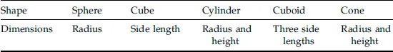
Regular-shaped particles can be accurately described by giving the shape and a number of dimensions. Examples are given in Table 1.1.

The description of the shapes of irregular-shaped particles is a branch of science in itself and will not be covered in detail here. Readers wishing to know more on this topic are referred to Hawkins (1993). However, it will be clear to the reader that no single physical dimension can adequately describe the size of an irregularly shaped particle, just as a single dimension cannot describe the shape of a cylinder, a cuboid or a cone. Which dimension we do use will in practice depend on (a) what property or dimension of the particle we are able to measure and (b) the use to which the dimension is to be put.

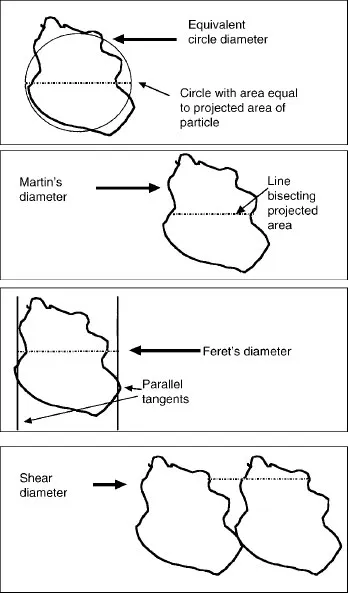
If we are using a microscope, perhaps coupled with an image analyser, to view the particles and measure their size, we are looking at a projection of the shape of the particles. Some common diameters used in microscope analysis are statistical diameters such as Martin’s diameter (length of the line which bisects the particle image), Feret’s diameter (distance between two tangents on opposite sides of the particle) and shear diameter (particle width obtained using an image shearing device) and equivalent circle diameters such as the projected area diameter (area of circle with same area as the projected area of the particle resting in a stable position). Some of these diameters are described in Figure 1.1. We must remember that the orientation of the particle on the microscope slide will affect the projected image and consequently the measured equivalent sphere diameter.

Table 1.1 Regular-shaped particles

Figure 1.1 Some diameters used in microscopy

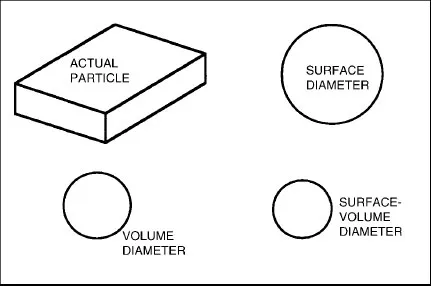
Figure 1.2 Comparison of equivalent sphere diameters

If we use a sieve to measure the particle size we come up with an equivalent sphere diameter, which is the diameter of a sphere passing through the same sieve aperture. If we use a sedimentation technique to measure particle size then it is expressed as the diameter of a sphere having the same sedimentation velocity under the same conditions. Other examples of the properties of particles measured and the resulting equivalent sphere diameters are given in Figure 1.2.

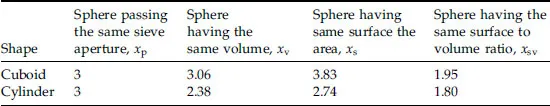
Table 1.2 compares values of these different equivalent sphere diameters used to describe a cuboid of side lengths 1, 3, 5 and a cylinder of diameter 3 and length 1.

The volume equivalent sphere diameter or equivalent volume sphere diameter is a commonly used equivalent sphere diameter. We will see later in the chapter that it is used in the Coulter counter size measurements technique. By definition, the equivalent volume sphere diameter is the diameter of a sphere having the same volume as the particle. The surface-volume diameter is the one measured when we use permeametry (see Section 1.8.4) to measure size. The surface-volume (equivalent sphere) diameter is the diameter of a sphere having the same surface to volume ratio as the particle. In practice it is important to use the method of size measurement which directly gives the particle size which is relevant to the situation or process of interest. (See Worked Example 1.1.)

Table 1.2 Comparison of equivalent sphere diameters

1.3 DESCRIPTION OF POPULATIONS OF PARTICLES

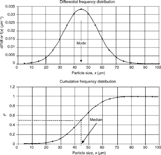
A population of particles is described by a particle size distribution. Particle size distributions may be expressed as frequency distribution curves or cumulative curves. These are illustrated in Figure 1.3. The two are related mathematically in that the cumulative distribution is the integral of the frequency distribution; i.e. if the cumulative distribution is denoted as F, then the frequency distribution dF/dx. For simplicity, dF/dx is often written as f(x). The distributions can be by number, surface, mass or volume (where particle density does not vary with size, the mass distribution is the same as the volume distribution). Incorporating this information into the notation, f_N(x) is the frequency distribution by number, f_S(x) is the frequency distribution by surface, F_S is the cumulative distribution by surface and F_M is the cumulative distribution by mass. In reality these distributions are smooth continuous curves. However, size measurement methods often divide the size spectrum into size ranges or classes and the size distribution becomes a histogram.

Figure 1.3 Typical differential and cumulative frequency distributions

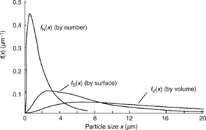
Figure 1.4 Comparison between distributions

For a given population of particles, the distributions by mass, number and surface can differ dramatically, as can be seen in Figure 1.4.

A fu...