Statistical Methods in Spatial Epidemiology

Andrew B. Lawson

• Editorial: Wiley
• Año: 2013
• ISBN:
  9781118723173
• Edición: 2
• Categoría: Medicine
• Categoría: Biostatistics

Spatial epidemiology is the description and analysis of the geographical distribution of disease. It is more important now than ever, with modern threats such as bio-terrorism making such analysis even more complex. This second edition of Statistical Methods in Spatial Epidemiology is updated and expanded to offer a complete coverage of the analysis and application of spatial statistical methods. The book is divided into two main sections: Part 1 introduces basic definitions and terminology, along with map construction and some basic models. This is expanded upon in Part II by applying this knowledge to the fundamental problems within spatial epidemiology, such as disease mapping, ecological analysis, disease clustering, bio-terrorism, space-time analysis, surveillance and infectious disease modelling.

• Provides a comprehensive overview of the main statistical methods used in spatial epidemiology.
• Updated to include a new emphasis on bio-terrorism and disease surveillance.
• Emphasizes the importance of space-time modelling and outlines the practical application of the method.
• Discusses the wide range of software available for analyzing spatial data, including WinBUGS, SaTScan and R, and features an accompanying website hosting related software.
• Contains numerous data sets, each representing a different approach to the analysis, and provides an insight into various modelling techniques.

This text is primarily aimed at medical statisticians, researchers and practitioners from public health and epidemiology. It is also suitable for postgraduate students of statistics and epidemiology, as well professionals working in government agencies.

Part I

The Nature of Spatial Epidemiology

1

Definitions, Terminology and Data Sets

Spatial epidemiology concerns the analysis of the spatial/geographical distribution of the incidence of disease. In its simplest form the subject concerns the use and interpretation of maps of the locations of disease cases, and the associated issues relating to map production and the statistical analysis of mapped data must apply within this subject. In addition, the nature of disease maps ensures that many epidemiological concepts also play an important role in the analysis. In essence, these two different aspects of the subject have their own impact on the methodology which has developed to deal with the many issues which arise in this area.

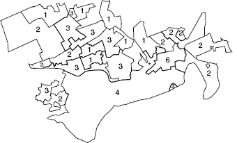
First, since mapped data are spatial in nature, the application of spatial statistical methods forms a core part of the subject area. The reason for this lies in the fact that the study of any data which are georeferenced (i.e. have a spatial/geographical location associated with them) may have properties which relate to the location of individual data items and also the surrounding data. For example, Figure 1.1 shows the total number of deaths from respiratory cancer found in 26 small areas (census tracts) in central Scotland over the period 1976–1983. This map displays a number of features which commonly arise when the geographical distribution of disease is examined. On this map the numbers (counts) of cases within each area are displayed. In some areas of the map the counts are similar to those found in the immediately surrounding areas (e.g. in the south and southeast of the map counts of 4 and 6 are recorded, while in the northwest of the map, lower counts are found in many areas). This similarity in the count data in groups of tracts is unlikely to have arisen from the allocation of a random sample of counts from a common statistical distribution. The counts may display some form of correlation in their levels based on their location, i.e. counts close to each other in space are similar. This form of correlation does not arise from the usual statistical models assumed to apply to independent observations found in, for example, clinical medical studies or other conventional statistical application areas. Hence, methods which apply to the analysis of these data must be able to address the possibility of such correlation existing in the mapped data under study. Another feature of this example, which commonly arises in the study of spatial epidemiology, is the irregular nature of the regions within which the counts are observed, i.e. the census tracts have irregular geographical boundaries. This may arise as a feature of the whole study region (study window) or may be found associated with tracts themselves. In some countries, notably in North America, small areas are often regular in shape and size and this feature simplifies the resulting analysis. However, in many other areas irregular region geometries are common. Finally, in some studies, the spatial distribution of cases or counts of disease are to be related to other locations on the map. For example, in Figure 1.1 the location of a potential (putative) environmental health hazard is also mapped (a metal-processing plant), and the focus of the study may be to assess the relationship of the disease incidence on the map to that location, perhaps to make inferences about the environmental risk in its vicinity.

Figure 1.1 Falkirk: central Scotland respiratory cancer counts in 26 census enumeration districts over a fixed time period. * Putative health hazard.

The second feature which uniquely defines the study of spatial epidemiology is that the mapped data are often discrete. Unlike other areas of spatial statistical analysis, which are often focused on continuous data, e.g. geostatistical methods, the data found in spatial epidemiology often take the form of point locations (the address locations of cases of disease) or counts of disease within regions such as census tracts or, at larger scale, counties or municipalities. Hence, the mapped data often consist of cartesian coordinates in the form of a grid reference or longitude/latitude of an address of a case, or a count of cases within a region with the associated location of that region (either as a point location of a centroid or as a set of boundary line segments defining the region). Given this form of data format, it is not surprising that models which have been developed for applications within this area are derived from stochastic point process theory (for case locations) and associated discrete probability distributions (for counts within arbitrary regions).

Finally, the epidemiological nature of these discrete spatial data leads to the derivation of models and methods which are related to conventional epidemiological studies. For example, the case–control study, where individual cases are matched to control individuals based on specific criteria, has parallels in spatial epidemiology where spatial control distributions are used to provide a locational control for cases. This is akin to the estimation of background hazard in survival studies. One fundamental epidemiological issue which arises in these studies is the incorporation of the local population which is at risk of contracting the disease in question. As we must control for the spatial variation in the underlying population, then we must be able to obtain good estimates of the population from which the cases or counts arise. This estimation often leads to the derivation of expected rates in the region count case and further to the estimation of the ratio of count to expected count/rate or the relative risk, in each area. Relative risk is a fundamental epidemiological concept (Clayton and Hills, 1993) in non-spatial epidemiological studies.

1.1 Map Hypotheses and Modelling Approaches

In any spatial epidemiological analysis, there will usually be a study focus which specifies the nature and style of the methods to be used. This focus will usually consist of a hypothesis or hypotheses about the nature of the spatial distribution of the disease which is to be examined, and it is convenient to categorise these hypotheses into three broad classes: disease mapping, ecological analysis and disease clustering. Usually, the distribution of cases of disease, whether in the form of counts or case address locations, can be thought to follow an underlying model, and the observed data may contain extra noise in the form of random variation around the model of interest. Often, the model will include aspects of the null (hypothesis) spatial distribution of the cases, which captures the ‘normal’ variation which is expected, and also aspects of the alternative spatial distribution. In much of spatial epidemiology, the focus of attention is on identifying features of the spatial distribution which are not captured by the null hypothesis distribution. This is mainly related to excess spatial aggregation of cases in areas of the map. That is, once the normal variation is allowed for, the residual spatial incidence above the normal incidence is the focus. Seldom is there any need to examine areas of lower aggregation than would be normally expected. Note that ‘normal’ variation is usually assumed to be defined by the underlying population distribution of the study region/window and cases are thought to arise in relation to the local variation in that distribution.

The first class, that of disease mapping, concerns the use of models to describe the overall disease distribution on the map. In disease mapping, often the object is simply to ‘clean’ the map of disease of the extra noise to uncover the underlying structure. In that situation, the null hypothesis could be that the case distribution arises from an unspecified or partly specified null spatial distribution (which includes the population spatial distribution) and the object is to remove the extra noise/variation. In this sense disease mapping is close in spirit to image processing where segmentation usually describes the process of allocating pixels or groups of pixels to classes.

The second class, that of ecological analysis, concerns the analysis of the relation between the spatial distribution of disease incidence and measured explanatory factors. This is usually carried out at an aggregated spatial level, and usually concerns regional incidence compared to explanatory factors measured at regional or other levels of aggregation (Greenberg et al., 1996). This contrasts with studies which use measurements made on individual subjects. However, many of the issues concerning interpretation of ecological studies are concerned with change in aggregation level and not aggregated data per se. For example, the ecological fallacy concerns making inference about individuals from analyses carried out at a higher scale, e.g. regional or country-wide level. Equally, the atomistic fallacy concerns making inferences about average characteristics from individual measurements. In what follows we assume a relatively wide definition of ecological, more in the sense of ecology itself, as any study which seeks to describe/explain the spatial distribution of disease based on the inclusion of explanatory variables. Two classic studies of this kind are presented by Cook and Pocock (1983), who examined the relation of cardiovascular incidence in the UK to a variety of variables (including water hardness, climate, location, socioeconomic and genetic factors and air pollution), and Donnelly (1995), who examined the respiratory health of school children and volatile organic compounds in the outdoor atmosphere. Note that this general definition can include the situation where case address locations are related to a pollution hazard via explanatory variables such as distance and direction from the hazard. In that case individual data are related to explanatory variables.

The final class, that of disease clustering, concerns the analysis of ‘unusual’ aggregations of disease, i.e. assessing whether there are any areas of elevated incidence of disease within a map. This type of analysis could take a variety of forms. First, the analysis could include the assessment of a complete map to ascertain whether the map is clustered. This is often termed general clustering. In this case, the null hypothesis would be that the disease map represents normal variation in incidence given the population distribution. The alternative hypothesis would include some specified clustering mechanism for the disease cases. This mechanism could be descriptive or include some notion of how the clusters form (e.g. clusters can form if infectious diseases are examined, and the contact rate of individuals can be modelled). General clustering is often treated as a form of autocorrelation and models for such effects are often employed. This form of clustering can be termed non-specific as it does not seek to determine where clusters are found but instead simply s...