Value Averaging

The Safe and Easy Strategy for Higher Investment Returns

Michael E. Edleson

• Editorial: Wiley
• Año: 2011
• ISBN:
  9781118044742
• Edición: 1
• Categoría: Business
• Categoría: Finance

Michael Edleson first introduced his concept of value averaging to the world in an article written in 1988. He then wrote a book entitled Value Averaging in 1993, which has been nearly impossible to find—until now. With the reintroduction of Value Averaging, you now have access to a strategy that can help you accumulate wealth, increase your investment returns, and achieve your financial goals.

1

Market Risk, Timing, and Formula Strategies

Whether you call it investing or playing the market, buying and selling stocks is risky business—risky but lucrative. In choosing to read this book, you have likely decided to build an investment portfolio that may include some of those risky stocks in order to garner some of those lucrative rewards. Before making investment decisions, you should have a reasonable idea of the typical risks you will face in the stock market and the likely rewards you might expect to earn. This chapter provides an introduction to these issues and familiarizes you with some historical data on market performance.

RISK AND MARKET RETURNS

First we will look at the investment returns that have been earned in the stock market in the past. Later in this section we discuss the risk inherent in these returns. Together, this information will provide you with a realistic sense of your opportunities in the stock market.

Market Returns over Time

When any wise market prognosticator is asked the inevitable question: Is the stock market going to move up or down?, the unsatisfying but correct answer is: Yes, it will. Day-to-day movements are anyone’s guess, but over time the market has risen substantially. Stock price movements for the past 66 years are shown in Figure 1-1.¹

Figure 1-1 MONTHLY STOCK PRICE LEVELS, 1926-1991

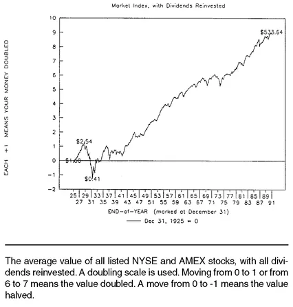
Note that a $1.00 investment on the last day of 1925 would have been worth $533.64 by the end of 1991. That’s a 9.98% compounded annual return over a period where inflation averaged 3.2%. Of course, you could have invested $2.54 prior to the October 1929 stock market crash and despaired as it went as low as $0.41 by mid-1932, losing over five-sixths of its value. Even though there has been only one such period in the past century, this scenario still highlights the magnitude of the potential risks faced when investing in the stock market.

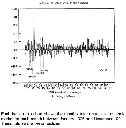
Figure 1-2 MONTHLY STOCK RETURNS, 1926-1991

If you (or more likely an ancestor) had invested $100 in the overall market each month during 1926-1991, your investment would have grown to $11,386,000, more than 140 times the total number of dollars you would have invested. Now admittedly, $100 a month was a lot of money back in the 1930s (worth about $800 in today’s dollars), but so is $11 million today. Let’s take a closer look at the type of risk entailed in attaining these investment rewards.

Figure 1-2 shows the total return (capital gains plus dividends) for each individual month in the 66-year period. Although it is extremely unusual for the market to move more than 20% in a given month, you can see that it has happened about ten times. The average market return for one month is slightly under +1.0% (0.95% monthly), or 12% annualized.² (See “Returns and Compounding” in the box on page 7.)

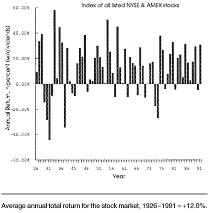
Figure 1-3 portrays similar data, but for years instead of months. Here it is easier to see that the market generally goes up, but that there is still random variability with no apparent pattern. The range of returns is from a − 44% loss to a +58% gain, although since World War II they fall in a tighter range of −28% to +51%. Individual stocks, of course, exhibit much more variability than the market as a whole, so avoid confusing typical market returns with what might happen to a single stock.

Figure 1-3 ANNUAL STOCK RETURNS, 1926-1991

RETURNS and COMPOUNDING

A return on investment (e.g., 8%) must be connected with a period of time (e.g., a year). Annual terms are commonly used, but not always. When we shift our concern from one time period to a different one, we must “translate” the return figure as well.

Suppose the total return on a 2-year investment was 21%. A natural way of stating this would be to convert the 2-year return into an annual figure—a 1-year return. But simply dividing the 21% by 2, yielding an annual return figure of 10.50%, would be incorrect. Simple “averaging” of a return ignores compounding. Suppose you had a $100 two-year investment, and made a 10.50% return on it in the first year. That gives you $110.50. With another 10.50% return in the second year, you end up with $122.10 (10.50% of $110.50 is $11.60). This is a 2-year return of 22.10%, not just 21 %. Actually, a 21% two-year return is equivalent to a 10% annual return ($100 + 10% = $110; $110 + 10% = $121, a 21 % total return).

If a is the annual return, then this formula will give you the compound return for n-years:

(1 + a)ⁿ = 1 + n-year return

In the example above, a = 10% and n = 2, so:

(1 + 0.10)² = 1.21 = 1 + n-year return
0.21 = 21 % = 2-year return

The process works in reverse, too, to find the annual return given a longerperiod return. Taking the n-th root (on a calculator, that’s raising something to the 1/n power), the formula is:

1 + a = ^{n-th root}(1 + n-year return)

or,

1 + a = (1 + n-year return)^1/n

EXAMPLE: What annual rate gets you a 50% return over five years?

1 + a = ^{5-th root}(1 + 0.50) = (1.50)^.2 = 1.0845
a = 8.45% annual return

This process can also be used for calculating compound returns for periods that are less than a year in length. Using the top formula, what is the monthly compound return if you get a 12% annual return? HINT: One month is ¹/₁₂ of one year.

(1 + 0.12)^1/12 = 1.0095 = 1 + monthly return
0.0095 = 0.95% = monthly return

A more general way to write the formula is helpful in translating monthly rates into annual. Suppose that your long time period is n times as long as your short time period. Then the per period compound returns are related as follows:

(1 + short period return)ⁿ = 1 + long period return

Suppose you could earn 1.0% each month on an investment. What is the annual return? Here, the short period return is 0.01, and n = 12:

(1.01)¹² = 1.1268 = 1 + long (annual) return
0.1268 = 12.68% = annual return

This is the proper method of converting between monthly and annual return figures, and it is used throughout this book.

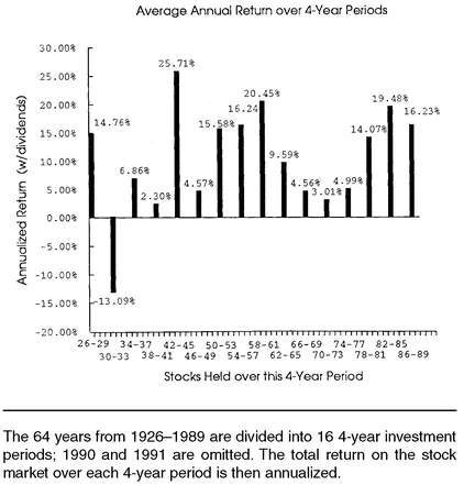
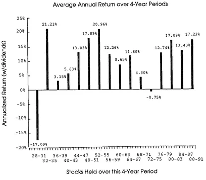
Even though the market is indeed risky, there is some truth to the statement Time heals all wounds. This is evident in Figure 1-4a, where instead of looking at one-year investments, we look at four-year periods. Only the worst period (the Great Depression) shows a loss. The annualized return over longer time periods is less variable, because the randomness of the returns causes them to “average out.”

Figure 1-4a ANNUALIZED STOCK RETURNS, 1926-1989

We could also look at the most recent 64 years, sliced into 4-year periods beginning in 1928. This similar analysis is shown in Figure 1-4b; the results differ slightly. While still less variable than single-year returns, these 4-year returns show a different pattern with more losses.

Figure 1-4b ANNUALIZED STOCK RETURNS, 1928-1991

Distribution of Market Returns

The risky nature of the stock market causes many people to mistakenly view it as a form of gambling. Yes, the outcome is uncertain and, as in a casino, you can lose your money. But in the stock market, the “house” doesn’t take a cut (although your broker or management company certainly will). On average, you will lose money in a casino; on average, you will win money or earn some positive return in the stock market (e.g., the +12% average noted above). In either case, the longer you “play,” the more certain these outcomes are. Also, unlike the potentially disappearing bankroll you take into the casino, there is no way the value of your diversified stock portfolio or fund will ever go to zero (even though any individual stock might).

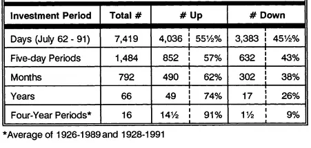
Let’s have a look at the historical data on market gains and losses—it is quite interesting and instructive. There were 792 months of market return data between 1926 and 1991; also, daily data were analyzed from the period July 1962 to December 1991. The results are tabulated in Table 1-1. Almost 55% of the daily returns were positive—in a typical 22-day month, the market would have had 12 up days and 10 down days. For longer periods, note the increasing probability of a gain in the market over that period.

The market tends to rise over time. Over just a brief instant of “market time,” this trend is indiscernible. Over a full day, you can see the tendency, but the random “bounce” around the trend still causes a large number (45½%) of down periods. But as we allow more time, the upward trend compounds, while at the same time the random bounces average each other out. So as time increases, we are more assured of getting a positive return out of the market. This characteristic of the market explains the typical advice from investment advisors to put into the stock market only your “five-year-andout” funds. That is, if you might need access to your funds within the next five years or sooner, it may not all still be there (if invested in the stock market) due to risk of loss; but funds invested for longer periods are less likely to experience a loss.

TABLE 1-1 Counting the Stock Market’s Ups and Downs

We can also look at the actual distribution of returns over various time periods to develop a better sense of th...