Production Management

Advanced Models, Tools, and Applications for Pull Systems

Yacob Khojasteh

• Editorial: Productivity Press
• Año: 2017
• ISBN:
  9781315394367
• Edición: 1
• Categoría: Business
• Categoría: Cultura aziendale

Inventory control is an essential task in production management. An effective inventory control can significantly reduce the holding cost and hence, total production cost. Selecting and implementing a suitable production control system plays an important role in inventory reduction and performance improvement of a production system. Since the introduction of Toyota's just-in-time philosophy, pull control systems have been adopted by numerous companies worldwide, both in the manufacturing and service sectors.

This book provides some recent developments in production management and presents modeling and analysis tools for pull production control systems. It contributes by combining theoretical findings and case study analysis results with a practical and contemporary view on how to effectively manage and control production systems.

Each chapter in this book focuses on a specific topic in production control systems, allowing readers to identify the chapters that relate to their interests. More specifically, the book is presented in three sections. The first section focuses on the design and implementation aspects of the pull production control systems, as well as performance evaluation approaches for pull systems. The second section presents a recent and comprehensive literature review. Three different case studies on implementation of pull production control systems are presented in the last section.

This book can be used as an essential source for students and scholars who need to specifically study the pull control systems. Since the superiority of these systems is controversial, the book can also provide an interesting and informative read for practitioners, managers, and employees who need to deepen their knowledge on pull production management systems.

DESIGN, IMPLEMENTAT ION, AND PERFORMANCE EVALUAT ION

I

Chapter 1

Pull Production Control Systems: Selection and Implementation Issues

Yacob Khojasteh

Contents

1.1 Introduction

1.2 Comparison Method

1.2.1 Analytical Comparisons

1.3 Numerical Experiments

1.3.1 An Example

1.3.1.1 Scenario 1

1.3.1.2 Scenario 2

1.4 Conclusions

References

1.1 Introduction

There are many studies regarding the evaluation and comparison of production control systems. Usually, two or more control systems are addressed and the superior system is highlighted, under certain conditions with a set of assumptions. Some studies propose a model or framework to conduct such comparisons. For example, Ghrayeb et al. (2009) compared push, pull, and hybrid control systems in an assemble-to-order manufacturing environment. They showed that in most cases, the hybrid system had the best performance. However, when the cost ratio of delivery lead time and inventory was small, the pull system performed better.

Gaury et al. (2000) compared Kanban, CONWIP, and hybrid control systems in a serial production line, and pointed out that the hybrid control system had the best performance. Pettersen and Segerstedt (2009) compared Kanban and CONWIP control systems through a simulation study over a small supply chain. They showed that the CONWIP control was superior to the Kanban with a higher throughput rate and the same amount of work-in-process (WIP) inventory. Khojasteh-Ghamari (2012) proposed a model for performance analysis of a production process controlled by Kanban and CONWIP. He showed the impact of initial inventories and card distribution as important parameters on system performance.

According to a survey by Framinan et al. (2003), comparing Kanban and CONWIP, many authors showed that CONWIP is superior to Kanban, when processing times on component operations in production processes are variable. However, a few studies, including Gstettner and Kuhn (1996) and Khojasteh-Ghamari (2009), reached the opposite conclusion. They showed that by choosing an appropriate number of cards at each workstation, Kanban could outperform CONWIP.

Bonvik et al. (1997) compared performance of different production control systems, with respect to WIP and service level, in a serial production line. They showed that CONWIP outperforms Kanban and Base-stock, with a high service level and lower WIP. However, as Framinan et al. (2003) mentioned, this result seems to be contradictory to the findings of Duenyas and Patana-anake (1998) as well as Paternina-Arboleda and Das (2001), which indicated that Base-stock outperforms CONWIP in a serial production line. These differing results highlight the need for more clarification and analysis. In this chapter, we address this controversy in generalizing the superiority among pull production control systems. For more literature reviews on the comparison of pull control systems, see Geraghty and Heavey (2006), Gonzlez-R et al. (2012), and Thürer et al. (2016).

Here, we introduce a comparison method (given in Section 1.2) followed by some numerical examples provided in Section 1.3 to briefly analyze the complexity in comparing the control systems.

1.2 Comparison Method

In this chapter, the framework proposed by Sato and Khojasteh-Ghamari (2012) is used for comparing pull production control systems in the presented example. For more details on the framework, which is based on the theory of token transactions systems, see Sato and Khojasteh-Ghamari (2012). In this section, we present a simple serial production process controlled by CONWIP to support the discussion and the numerical example provided in the next section.

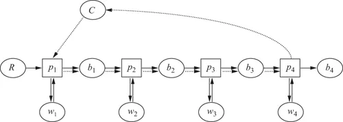
We can consider a simple production process with four workstations. The activity interaction diagram (AID) of this production process controlled by CONWIP is depicted in Figure 1.1. See Sato and Praehofer (1997) for definitions and concepts of the AID.

Figure 1.1 A serial production process with four workstations controlled by CONWIP (Sato and Khojasteh-Ghamari, 2012).

Raw material R is being processed through p ₁ to p ₄ and at the end, it is stored in the place b ₄ as finished products, while b _i (i = 1,…,4) is the output buffer of station i, and w _i (i = 1,…,4) represents the worker/operator/machine of station i. Queue C contains CONWIP cards. Solid lines represent material flows and dashed lines indicate card/information flows.

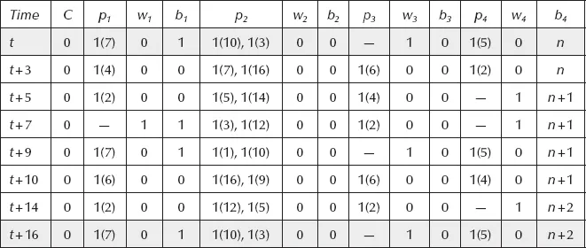
The system reaches a steady state after a sufficient period of time. We can show the steady state of the system by referring to the state transition table (Sato and Praehofer, 1997). At steady state, the system shows a periodic behavior. Table 1.1 shows part of the state transition table for the CONWIP controlled production system depicted in Figure 1. Processing time at p ₁ to p ₄ is set to 7, 16, 6, and 5, respectively. Process p ₂ has two workers, while the others have one each. Initial inventory in each buffer is set to zero. With this structure, at least four cards are needed to circulate in the entire system to enable maximum throughput. In this table, “—” represents there is no part being processed, that the corresponding worker is idle. For example, “1(7),” shows that one part is being processed and it will finish after 7 time units.

Table 1.1 State Transition Table of the CONWIP Example

The numbers and symbols in the first row of the state transition table, given in Table 1.1, can be interpreted as follows. At time t, there is no available card in the card buffer C (C = 0). One part is being processed at p ₁, which will finish after 7 time units. Since a part is being processed at p ₁, the corresponding worker w ₁ is busy and is not available (w ₁ = 0). There is one part in the first output buffer (b ₁ = 1), and two parts are being processed at p ₂, one will finish after 10 time units and the other after 3 time units. Hence, none of the respective workers is available (w ₂ = 0). No part is in the output buffer of the second and third stations (b ₂ = b ₃ = 0), also no part is being processed at p ₃. Therefore, the respective worker is idle (w ₃ = 1). One part is being processed in p ₄ with a remaining time of 5 time units causing its worker to be busy (w ₄ = 0). In the last output buffer b ₄ waiting to be delivered to the customer, n finished products are available.

After 3 time units (which is the smallest remaining time at time t), p ₂ finishes one part. This means that the current time is now t + 3, as shown in the second row of the table. At this ...