Probabilistic Methods in Geotechnical Engineering

Proceedings of the conference, Canberra, 10-12 February 1993

K.S. Li, S.-C.R. Lo, K.S. Li, S.-C.R. Lo

• Editorial: CRC Press
• Año: 2020
• ISBN:
  9781000150452
• Edición: 1
• Categoría: Tecnologia e ingegneria
• Categoría: Agronomia

The proceedings of this conference contain keynote addresses on recent developments in geotechnical reliability and limit state design in geotechnics. It also contains invited lectures on such topics as modelling of soil variability, simulation of random fields and probability of rock joints.

Contents: Keynote addresses on recent development on geotechnical reliability and limit state design in geotechnics, and invited lectures on modelling of soil variability, simulation of random field, probabilistic of rock joints, and probabilistic design of foundations and slopes. Other papers on analytical techniques in geotechnical reliability, modelling of soil properties, and probabilistic analysis of slopes, embankments and foundations.

Invited lectures

Simulation of random fields

A.M.Hasofer
University of New South Wales, Sydney, N.S.W., Australia

ABSTRACT: A number of algorithms which have been recently developed for simulating stationary zero-mean Gaussian random fields with given spectral density will be described. The two main approaches are the frequency-domain and the spatial domain discretizations. The method of turning bands for the simulation of isotropic fields and an interpolation algorithm based on the sampling theorem will also be described.

1. INTRODUCTION

Data description in geotechnical problems usually involves irreducible uncertainties which can only be quantified in probabilistic terms. Because soil is, by its very nature, a three-dimensional continuum, we are led to model its properties by random fields. In specific circumstances, the dimension of the field can be reduced to two or even one.

But it is a general truth that the solution of design problems in geotechnical engineering is far easier in a deterministic context than in a probabilistic one. In fact, exact, or even approximate solutions of probabilistic problems are usually beyond the reach of our present mathematical techniques, unless the models are linear and the variables Gaussian.

With the advent of powerful computers, it has become feasible to circumvent the above difficulty by the use of simulation. A number of realizations of the random field that models the data are generated, and for each realization the deterministic problem is solved. From the set of solutions obtained, inferences about the design parameters can then be made. The optimum design can finally be chosen by appropriately balancing safety and cost.

However, unless the simulation of the random field is carefully planned, it can be very costly in computer time, and moreover the simulations may introduce crude errors which lead to misleading results. This is particularly true when the choice of the design depends on the evaluation of small failure probabilities. In this paper, a number of methods of random field simulation which have been proposed and used over past years will be described. The topic is still at a pioneering stage. Until a serious benchmark study of the various proposed methods is carried out, choosing the appropriate method for a particular problem will remain the responsibility of the individual researcher.

Attention will be restricted to stationary fields with zero mean.

2. GAUSSIAN VERSUS NON-GAUSSIAN FIELDS

It was mentioned in the previous section that the assumption of Gaussianity considerably simplifies stochastic problems. Indeed, all the simulation methods which we shall describe produce fields which are either exactly or approximately Gaussian.

In general, however, geotechnical random fields may well be far away from Gaussianity.

To understand the rationale of the current approach to this problem one must recollect how the probabilistic structure of a random field is specified. A full specification requires that all n—dimensional joint distribution functions at n arbitrary points in the field for all n = 1,2,3,... be given. As against this, a Gaussian field only requires specification of the mean at each point and the covariance function at each pair of points.

Now the determination of multivariate non-Gaussian distributions is usually quite impractical. So what is usually done is simply to adjust the marginal distributions of the field to conform to the required specification. Matheron (1973) calls such an adjustment an “anamorphosis”.

For example, suppose that the field X(t) we must simulate is stationary, has marginal distributions F(x) and two-dimensional distributions G(x,y). Let $(x) be the distribution function of the standard normal distribution. Then

is a standard normal variable for each t.

We calculate

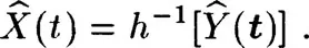
and then simulate a Gaussian random field Ŷ(t) with zero mean and covariance function R(t). Finally we set

The field

(t) has the specified marginal distribution F and in addition h(

) has the correct covariance. Experience shows that the field

closely simulates the required field X.

3. CONTINUOUS VERSUS DISCRETE FIELDS

Let X(t) be the random field to be simulated. The parameter t is a vector of length three (or sometimes only of length two or even one). The domain of t can be the full corresponding Euclidian space. We then speak of a continuous field. Alternatively it can be the set of lattice points (with appropriate scales on the axes). We then speak of a discrete field. Of course when a simulation is carried out on a computer we can only simulate at a finite number of points. But when the simulation is continuous the points can be chosen arbitrarily near to each other, while with discrete fields the points are chosen in advance. Moreover, with a formula for continuous simulation one can often carry out various analytical operations such as integration and differentiation. This cannot be done with formulae for discrete simulation.

4. THE INTERPOLATION FORMULA

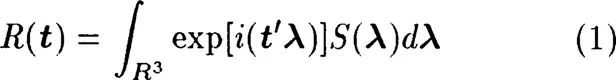
Suppose that X(t) is a continuous zero-mean stationary Gaussian field with covariance function

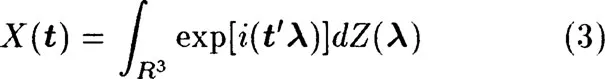
Then we have the representation

where t′λ is the scalar product of t and λ, S(λ) is the spectral density of X(t), and dλ = dλ₁dλ₂ dλ₃.

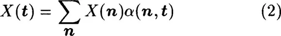
Suppose that the field is band-limited, i.e. that S(λ) = 0 outside a cube of side (−2πβ,2πβ). Let n represent the lattice points in the field at a distance 1/2β on each axis. According to the sampling theorem, the values of X(t) at the points n determine the whole field X(t). In fact X(t) is given by the formula

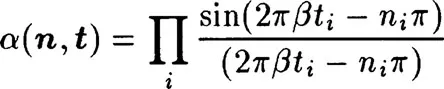
where the summation extends over all lattice points. The kernel α(n,t) is given, for t = (t₁,t₂, t₃) by

if n = (n₁/2β, n₂/2β, n₃/2β), in the case of a three-dimensional field, with similar formulae in other cases.

If the band-limited property holds the interpolation formula enables us to convert a discrete random field to a continuous one. In practice, this is almost always the case. (Gregoriu and Balopoulou 1992. See also Hasofer 1990).

5. METHODS OF SIMULATION

There are two fundamental types of simulation:

(a) Discretization in the frequency domain.

(b) Discretization in the spatial domain.

(a) The frequency domain

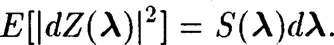
To the representation (1) of the covariance there corresponds a representation of the field X(t) as a stochastic integral

where Z(λ) is a field with orthogonal increments and

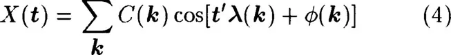
Simulation is carried out by discretizing formula (3) and taking the real part, in the form

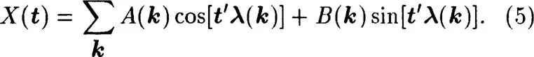
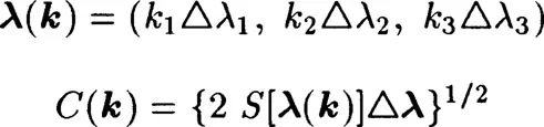
where the summation is over all triples k = (k₁,k₂,k₃) of integers such that |k_i| ≤ N_i;i = 1,2,3. Alternatively (3) can be written as

Two methods have been proposed for choosing the stochastic element in the model: the random phase method and the random amplitude method.

(i) The random phase method. (See e.g. Shinozuka 1987).

In equation (4) we take

and the ϕ(k) are independent random variables uniformly distributed over (0,27π). It is easy to ...