Mathematics
Confidence Interval for Population Proportion
A confidence interval for a population proportion is a range of values within which we are reasonably confident the true population proportion lies. It is calculated using sample data and provides a measure of the uncertainty associated with estimating the population proportion. The confidence interval is often expressed as a percentage, such as 95% confidence.
Written by Perlego with AI-assistance
Related key terms
1 of 5
10 Key excerpts on "Confidence Interval for Population Proportion"
 eBook - PDF
- Roxy Peck, Chris Olsen, , Tom Short, Roxy Peck, Chris Olsen, Tom Short(Authors)
- 2019(Publication Date)
- Cengage Learning EMEA(Publisher)
A Bootstrap Confidence Interval for a Population Proportion When a sample proportion p / is used to estimate a population proportion, we know that the value of p / is not likely to be exactly equal to the value of the population proportion. But if the sample is selected in a reasonable way, we expect that the value of p / will be somewhere around the value of the population proportion. A confidence interval quantifies what is meant by “around the value of the population proportion.” When the assumptions of the large-sample confidence interval are reasonable, the confidence interval based on a sampling distribution of p / that is approximately normal can be used to determine the larg-est value that the difference between the observed sample proportion and the actual value of the population proportion is likely to be for a specific confidence level. However, sometimes the distribution of p / is not approximately normal. In this case, constructing a confidence interval still requires knowing something about how far away the sample proportion is likely to be from the value of the population proportion. For example, suppose that the sample proportion is p / 5 0.32 and that it is unlikely to be smaller than the actual value of the population proportion by more than 0.04. Then we think that the population proportion is less than 0.36 (from 0.32 1 0.04). If it is also unlikely that the sam-ple proportion is greater than the population proportion by more than 0.05, then we could say that we think that the population proportion is greater than 0.27 (from 0.32 2 0.05). A reasonable interval estimate of the population proportion based on the sample would then be (0.27, 0.36). Bootstrapping is a way to determine what number to add and what number to subtract from the sample proportion to form a confidence interval. No longer available |Learn more
- Jessica Utts, Robert Heckard(Authors)
- 2015(Publication Date)
- Cengage Learning EMEA(Publisher)
Estimating Proportions with Confidence 383 10.2 CI Module 1: Confidence Intervals for Population Proportions The material in this module is divided into three lessons. Lesson 1 explains how to implement the general formula to find a confidence interval for a population proportion for any confidence level. Lesson 2 explains why the formula works. In Lesson 3, we reconcile the formulas in this chapter with the confidence interval formula in Chapter 5, in which we added and subtracted a margin of error of 1 n to the sample proportion to find an approximate 95% confidence interval for a population proportion. We also explain why the media reports this margin of error. Lesson 1: Details of How to Compute a Confidence Interval for a Population Proportion The confidence interval method described in this section is applicable to a surprisingly wide range of interesting research questions. The scenarios are similar to the ones that we encountered when we studied binomial random variables in Chapter 8. There are two common settings in which we might want to estimate a population proportion or probability p : 1. A population exists, and we are interested in knowing what proportion of it has a certain trait, opinion, characteristic, response to a treatment, and so on. Two typi-cal research questions for this setting follow: • What proportion of drivers are talking on a cell phone at any given moment? • What proportion of a population of smokers would quit smoking if they were to wear a nicotine patch for 8 weeks? 2. A repeatable situation exists, and we are interested in the long-run probability of a specific outcome .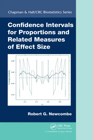
- Robert Gordon Newcombe(Author)
- 2012(Publication Date)
- CRC Press(Publisher)
On the other hand, the support scale for a proportion is bounded: by definition a proportion has to lie between 0 and 1, yet the simplest confidence interval suffers from the deficiency that calculated lower or upper limits can fall out-side this range. Furthermore, in the continuous case, the true population mean μ , the sam-pled observations y 1 , y 2 , … , y n and the sample mean y can all take any value on a continuous scale. Likewise, when we are considering proportions, the population proportion π can take any value between 0 and 1. In contrast, the random variable R representing the number of individuals who turn out to be positive can only take a discrete set of possible values r = 0, 1, 2, … , n – 1 or n . Consequently, the sample proportion p can only take one of a discrete set of values, 0, 1/ n , 2/ n , … , ( n – 1)/ n or 1. As a consequence of discreteness and boundedness, the simplest calcula-tion methods for proportions generally do not perform adequately, and better methods are required. Furthermore, similar issues affect interval estimation for other quantities related to proportions, to a greater or lesser degree. See Newcombe (2008c) for a general discussion of some of the issues in relation to proportions and their differences. The methods recommended throughout this book are designed to obviate the deficiencies of the simplest methods. 3.2 The Wald Interval The simplest confidence interval for a proportion in scientific use is con-structed in much the same way as the confidence interval for a mean, based on the standard error. The formula usually used to calculate the simple asymptotic interval is p ± z × SE( p ). Here, p denotes the empirical estimate of the proportion, r / n , with standard error SE( p ) = √ ( pq / n ), q denotes 1 – p and z denotes the appropriate centile of the standard Gaussian distribution, 1.960 for the usual two-sided 95% interval. eBook - PDF
- Barbara Illowsky, Susan Dean(Authors)
- 2016(Publication Date)
- Openstax(Publisher)
Businesses that sell personal computers are interested in the proportion of households in the United States that own personal computers. Confidence intervals can be calculated for the true proportion of stocks that go up or down each week and for the true proportion of households in the United States that own personal computers. The procedure to find the confidence interval, the sample size, the error bound, and the confidence level for a proportion is similar to that for the population mean, but the formulas are different. How do you know you are dealing with a proportion problem? First, the underlying distribution is a binomial distribution. (There is no mention of a mean or average.) If X is a binomial random variable, then X ~ B(n, p) where n is the number of trials and p is the probability of a success. To form a proportion, take X, the random variable for the number of successes and divide it by n, the number of trials (or the sample size). The random variable P′ (read "P prime") is that proportion, P′ = X n 456 Chapter 8 | Confidence Intervals This OpenStax book is available for free at http://cnx.org/content/col11562/1.17 (Sometimes the random variable is denoted as P ^ , read "P hat".) When n is large and p is not close to zero or one, we can use the normal distribution to approximate the binomial. X ~ N(np, npq ) If we divide the random variable, the mean, and the standard deviation by n, we get a normal distribution of proportions with P′, called the estimated proportion, as the random variable. (Recall that a proportion as the number of successes divided by n.) X n = P′ ~ N ⎛ ⎝ np n , npq n ⎞ ⎠ Using algebra to simplify : npq n = pq n P′ follows a normal distribution for proportions: X n = P′ ~ N ⎛ ⎝ np n , npq n ⎞ ⎠ The confidence interval has the form (p′ – EBP, p′ + EBP). eBook - PDF
- Prem S. Mann(Author)
- 2017(Publication Date)
- Wiley(Publisher)
Confidence interval An interval constructed around the value of a sample statistic to estimate the corresponding population parameter. Confidence level Confidence level, denoted by (1 − α)100%, that states how much confidence we have that a confidence interval con- tains the true population parameter. Degrees of freedom (df) The number of observations that can be chosen freely. For the estimation of μ using the t distribution, the degrees of freedom is n − 1. Estimate The value of a sample statistic that is used to find the corresponding population parameter. Estimation A procedure by which a numerical value or values are assigned to a population parameter based on the information collected from a sample. GLOSSARY sample, will you conclude that the machine needs an adjustment? Assume that the lengths of all such rods have an approximate normal distribution. 8.80 A hospital administration wants to estimate the mean time spent by patients waiting for treatment at the emergency room. The waiting times (in minutes) recorded for a random sample of 32 such patients are given below. 110 42 88 19 35 76 10 151 2 44 27 77 53 102 66 39 20 108 92 55 14 52 3 62 78 15 60 121 40 35 11 72 Construct a 98% confidence interval for the corresponding population mean. Use the t distribution. 8.81 A travel magazine wanted to estimate the mean amount of leisure time per week enjoyed by adults. The research department at the mag- azine took a sample of 36 adults and obtained the following data on the weekly leisure time (in hours). 15 12 18 23 11 21 16 13 9 19 26 14 7 18 11 15 23 26 10 8 17 21 12 7 19 21 11 13 21 16 14 9 15 12 10 14 Construct a 99% confidence interval for the mean leisure time per week enjoyed by all adults. Use the t distribution. 8.82 A drug that provides relief from headaches was tried on 18 ran- domly selected patients. eBook - PDF
- Prem S. Mann(Author)
- 2016(Publication Date)
- Wiley(Publisher)
Confidence level Confidence level, denoted by (1 − α)100%, that states how much confidence we have that a confidence interval con- tains the true population parameter. Degrees of freedom (df) The number of observations that can be chosen freely. For the estimation of μ using the t distribution, the degrees of freedom is n − 1. Estimate The value of a sample statistic that is used to find the corresponding population parameter. Estimation A procedure by which a numerical value or values are assigned to a population parameter based on the information collected from a sample. Glossary 338 Chapter 8 Estimation of the Mean and Proportion per year with a standard deviation of $74. Assuming that the life insurance policy premiums for all life insurance policyholders have an approximate normal distribution, make a 99% confidence interval for the population mean, μ. 8.77 A survey of 500 randomly selected adult men showed that the mean time they spend per week watching sports on television is 9.75 hours with a standard deviation of 2.2 hours. Construct a 90% confidence interval for the population mean, μ. 8.78 A random sample of 300 female members of health clubs in Los Angeles showed that they spend, on average, 4.5 hours per week doing physical exercise with a standard deviation of .75 hour. Find a 98% confidence interval for the population mean. 8.79 A computer company that recently developed a new software product wanted to estimate the mean time taken to learn how to use this software by people who are somewhat familiar with computers. A random sample of 12 such persons was selected. The following data give the times (in hours) taken by these persons to learn how to use this software. 1.75 2.25 2.40 1.90 1.50 2.75 2.15 2.25 1.80 2.20 3.25 2.60 Construct a 95% confidence interval for the population mean. Assume that the times taken by all persons who are somewhat familiar with computers to learn how to use this software are approximately nor- mally distributed. eBook - PDF
- Prem S. Mann(Author)
- 2020(Publication Date)
- Wiley(Publisher)
• Explain various alternatives for decreasing the width of a confidence interval. • Determine the minimum sample size to produce a confidence interval for p with a predetermined margin of error. Often we want to estimate a population proportion or percentage. (Recall that a percentage is obtained by multiplying the proportion by 100.) For example, the production manager of a company may want to estimate the proportion of defective items produced on a machine. A bank manager may want to find the percentage of customers who are satisfied with the service provided by the bank. Again, if we can conduct a census each time we want to find the value of a population proportion, there is no need to learn the procedures discussed in this section. However, we usually derive our results from sample surveys. Hence, to take into account the variability in the results obtained from different sample surveys, we need to know the procedures for esti- mating a population proportion. Recall from Chapter 7 that the population proportion is denoted by p, and the sample proportion is denoted by p ̂ . This section explains how to estimate the population proportion, p, using the sample proportion, p ̂ . The sample proportion, p ̂ , is a sample statistic, and it possesses a sampling distribution. From Chapter 7, we know that: 1. The sampling distribution of the sample proportion p ̂ is approximately normal for a large sample. In the case of a proportion, a sample is considered to be large if np > 5 and nq > 5. 2. The mean of the sampling distribution of p ̂ , μ p ̂ , is equal to the population proportion, p. 3. The standard deviation of the sampling distribution of p ̂ is σ p ̂ = √ _ pq/ n , where q = 1 − p, given that n __ N ≤ .05. To reiterate, in the case of a proportion, a sample is considered to be large if np and nq are both greater than 5. If p and q are not known, then np ̂ and nq ̂ should each be greater than 5 for the sample to be large. eBook - ePub
Social Statistics
Managing Data, Conducting Analyses, Presenting Results
- Thomas J. Linneman(Author)
- 2017(Publication Date)
- Routledge(Publisher)
Chapter 5 Using a Sample Mean or Proportion to Talk About a Population Confidence IntervalsThis chapter covers ...
- . . . building a probability distribution of sample means
- . . . how to find and interpret the standard error of a sampling distribution
- . . . what the Central Limit Theorem is and why it is important
- . . . population claims and how to put them to the test
- . . . how to build and interpret confidence intervals
- . . . how a researcher used confidence intervals to study popular films
- . . . how researchers used confidence intervals to study Uber and traffic fatalities
Introduction
In this chapter we continue our exploration of inference, going through some procedures that you will find strikingly similar to those in the chi-square chapter. Whereas in the chi-square chapter we dealt with variables of the nominal or ordinal variety, here we deal with ratio-level variables. Our attention turns away from sample crosstabs and toward sample means (and, at the end of the chapter, proportions). But keep in mind that the inference goal remains the same: we will use sample means in order to make claims about population means. Just as we talked about the chi-square probability distribution, we’ll start this chapter with a distribution of sample means.Sampling Distributions of Sample Means
Imagine a hypothetical class with 100 students in it. These students will serve as our population: it is the entire group of students in which we are interested. They get the following hypothetical grades:■ Exhibit 5.1: Grades for a Population of 100 Students: Frequency DistributionHere is a bar graph of this frequency distribution:Grade # of Students Receiving This Grade 1.0 1 1.1 1 1.2 1 1.3 2 1.4 2 1.5 2 1.6 2 1.7 3 1.8 3 1.9 3 2.0 4 2.1 4 2.2 5 2.3 6 2.4 7 2.5 8 2.6 7 2.7 6 2.8 5 2.9 4 3.0 4 3.1 3 3.2 3 3.3 3 3.4 2 3.5 2 3.6 2 3.7 2 3.8 1 3.9 1 4.0 1 Source: Hypothetical data. eBook - PDF
Statistics, Student Solutions Manual
Unlocking the Power of Data
- Robin H. Lock, Patti Frazer Lock, Kari Lock Morgan, Eric F. Lock, Dennis F. Lock(Authors)
- 2021(Publication Date)
- Wiley(Publisher)
One set of 1000 bootstrap proportions is shown in the figure below. For a 95% confidence interval we need to find the 2.5%-tile and 97.5%-tile, leaving 95% of the distribution in the middle. For this distribution those points are at 0.664 and 0.776, so we are 95% sure that the proportion in the population who agree is between 0.664 and 0.776. Answers will vary slightly for different simulations. 3.123 The sample proportion who agree is ˆ p = 382/1000 = 0.382. One set of 1000 bootstrap proportions is shown in the figure below. For a 99% confidence interval we need to find the 0.5%-tile and 99.5%-tile, leaving 99% of the distribution in the middle. For this distribution those points are at 0.343 and 0.423, so we are 99% sure that the proportion in the population who agree is between 0.343 and 0.423. Answers will vary slightly for different simulations. 76 CHAPTER 3 3.125 The 98% confidence interval uses the 1%-tile and 99%-tile from the bootstrap means. We are 98% sure that the mean number of penalty minutes for NHL players in a season is between 14.3 and 36.7 minutes. 3.127 After creating the bootstrap distribution, we use the boundaries for the middle 90% of bootstrap statistics to find the confidence interval. The 90% confidence interval is about 0.58 to 0.81. We are 90% confident that the proportion of all college instructors who are bothered by student off-task phone use during class is between 0.58 and 0.81. 3.129 Using StatKey or other technology, we produce a bootstrap distribution such as the figure shown below. For a 99% confidence interval, we find the 0.5%-tile and 99.5%-tile points in this distribution to be 0.467 and 0.493. We are 99% confident that the percent of all Europeans (from these nine countries) who can identify arm or shoulder pain as a symptom of a heart attack is between 46.7% and 49.3%. Since every value in this interval is below 50%, we can be 99% confident that the proportion is less than half. eBook - PDF
Biostatistics
Basic Concepts and Methodology for the Health Sciences, 10th Edition International Student Version
- Wayne W. Daniel, Chad L. Cross(Authors)
- 2014(Publication Date)
- Wiley(Publisher)
19. A certain drug was found to be effective in the treatment of pulmonary disease in 180 of 200 cases treated. Construct the 90 percent confidence interval for the population proportion. 20. Seventy patients with stasis ulcers of the leg were randomly divided into two equal groups. Each group received a different treatment for edema. At the end of the experiment, treatment effectiveness was measured in terms of reduction in leg volume as determined by water displacement. The means and standard deviations for the two groups were as follows: Group (Treatment) " x s A 90 cc 25 B 120 cc 30 Construct a 90 percent confidence interval for the difference in population means. 21. What is the average serum bilirubin level of patients admitted to a hospital for treatment of hepatitis? A sample of 10 patients yielded the following results: 20:5; 14:8; 21:3; 12:7; 15:2; 26:6; 23:4; 22:9; 15:7; 19:2 Construct a 95 percent confidence interval for the population mean. 206 CHAPTER 6 USING SAMPLE DATA TO MAKE ESTIMATES ABOUT POPULATION PARAMETERS 22. Determinations of saliva pH levels were made in two independent random samples of seventh-grade schoolchildren. Sample A children were caries-free while sample B children had a high incidence of caries. The results were as follows: A: 7.13, 7.10, 7.63, 7.99, 7.20, 7.15, 7.92 7.24, 7.86, 7.47, 7.82, 7.37, 7.66, 7.62, 7.65 B: 7.36, 7.04, 7.19, 7.41, 7.10, 7.15, 7.36, 7.46, 7.60, 7.01, 7.20, 7.21 Construct a 90 percent confidence interval for the difference between the population means. Assume that the population variances are equal. 23. Drug A was prescribed for a random sample of 12 patients complaining of insomnia. An independent random sample of 16 patients with the same complaint received drug B.
Index pages curate the most relevant extracts from our library of academic textbooks. They’ve been created using an in-house natural language model (NLM), each adding context and meaning to key research topics.