Matrix Determinant

11 Key excerpts on "Matrix Determinant"

• 

  No longer available |Learn more

  Elementary Linear Algebra & Vector Mathematics (Concepts & Applications)

  • (Author)
  • 2014(Publication Date)
  • Library Press

    (Publisher)

  ________________________ WORLD TECHNOLOGIES ________________________ Chapter 4 Determinant and Coordinate Vector Determinant In algebra, the determinant is a special number associated with any square matrix. The fundamental geometric meaning of a determinant is a scale factor or coefficient for measure when the matrix is regarded as a linear transformation. Thus a 2 × 2 matrix with determinant 2 when applied to a set of points with finite area will transform those points into a set with twice the area. Determinants are important both in calculus, where they enter the substitution rule for several variables, and in multilinear algebra. When its scalars are taken from a field F , a matrix is invertible if and only if its determinant is nonzero; more generally, when the scalars are taken from a commutative ring R , the matrix is invertible if and only if its determinant is a unit of R . Determinants are not that well-behaved for noncommutative rings. The determinant of a matrix A is denoted det( A ), or without parentheses: det A . An alternative notation, used for compactness, especially in the case where the matrix entries are written out in full, is to denote the determinant of a matrix by surrounding the matrix entries by vertical bars instead of the usual brackets or parentheses. Thus denotes the determinant of the matrix For a fixed nonnegative integer n , there is a unique determinant function for the n × n matrices over any commutative ring R . In particular, this unique function exists when R is the field of real or complex numbers. ________________________ WORLD TECHNOLOGIES ________________________ Interpretation as the area of a parallelogram The area of the parallelogram is the absolute value of the determinant of the matrix formed by the vectors representing the parallelogram's sides. The 2×2 matrix has determinant

  Sign up to read

  Learn more about book
• 

  eBook - ePub

  Engineering Mathematics with Applications to Fire Engineering

  • Khalid Khan, Tony Lee Graham(Authors)
  • 2018(Publication Date)
  • CRC Press

    (Publisher)

  4 Determinants and Matrices

  4.1 Background

  Matrices with different dimensions are a standard method for solving a wide range of problems in many disciplines. In science and engineering, when considering particular problems, the derivation of the solutions to these problems can come down to solving a system of linear equations. In this chapter, different methods for solving a linear system of equations will be discussed and these methods involve the concepts of determinants and matrices.

  4.2 Introduction to Determinants

  Determinants arise naturally in the solution of a set of linear equations. Also they will help solve linear equations using the matrix inversion method (see Section 4.3.6 ). Starting with a general set of two linear simultaneous equations as follows:

  a x + b y = e

  4.1

  4.1

  c x + d y = f

  4.2

  4.2

  where a , b , c , d , e , and f are constants. How do you find the values of x and y ? Since the values of a , b , c , and d are not known, all that can be done is try to eliminate either x or y .

  If one decides to get rid of y , then to make the coefficients of y the same, first multiply Equation 4.1 by d and Equation 4.2 by b :

  a d x + b d y = d e

  4.3

  4.3

  b c x + b d y = b f

  4.4

  4.4

  Then subtracting Equation 4.4 from Equation 4.3 :

  a d x − b c x = d e − b f   ∴   x ( a d − b c ) = d e − b f   ∴   x =

  d e − b f

  a d − b c

  A similar approach, getting rid of x , would give the result as

  y =

  a f − c e

  a d − b c

  Now provided that the denominator term ad − bc ≠ 0, then a symbol can be used to define a 2-by-2 determinant using parallel lines (∣ ∣), as shown next:

  |

  a b

  c d

  |

  ≜ a d − b c

  4.5

  4.5

  Note:The symbol ≜ means “defined as.”

  This definition given by Equation 4.5 is just the difference in product of the diagonals.

  Notice also how these answers for x and y

  Sign up to read

  Learn more about book
• 

  eBook - PDF

  Mathematical Techniques in GIS

  • Peter Dale(Author)
  • 2014(Publication Date)
  • CRC Press

    (Publisher)

  134 Mathematical Techniques in GIS 7.2 DETERMINANTS The number ( ae – bd ) that was used above to scale the whole multiplication to make the diagonal numbers all equal to 1 is a special number for the 2 * 2 matrix A that is called its determinant . This is usually written with straight-line brackets so that: = = = -a b d e ae bd The determinant of | | . A A The notation should not be confused with the idea of a modulus , which also uses straight-line brackets. The modulus (or “mod”) of a value is a positive real number that is the absolute value of a quantity, that is, regardless of whether mathematically it is positive or negative. Thus, mod (–3) = |–3| = + 3. A determinant is always a square matrix with n rows and n columns, n being an integer such as 1, 2, 3, 4, and so on. If it happens in a 2 * 2 matrix that ae = bd , then 1/| A | = 1/0 which is infinite, hence the matrix A has no inverse. The matrix is then said to be singular . For a 3 * 3 matrix the process is slightly more complicated. The calculation is broken down into three stages where = a b c d e f g h i a e f h i b d f g i c d e g h three parts . . . . and . . . . and . . . . Each of these subcomponents contains a 2 * 2 determinant that is known as the minor of the element in the first row. The value of the 3 * 3 determinant (Box 7.3 and Example 7.3) is then defined as: | A | = a ( ei – fh ) – b ( di – fg ) + c ( dh – eg ) Note the alternating signs, plus a , minus b , plus c , and so forth. EXAMPLE 7.2: MATRIX INVERSE If A is a 3 * 3 matrix 1 4 3 2 5 4 7 6 7 and B = 5.5 5 0.5 7 7 1 11.5 11 1.5 − − − − − then A B B A * 1 0 0 0 1 0 0 0 1 * = = A * B = I the identity matrix and hence B = A –1 , the inverse of A . 135 Matrices and Determinants If for instance two (or more) rows (or columns) differ by a common factor, then | A | will be zero.

  Sign up to read

  Learn more about book
• 

  eBook - PDF

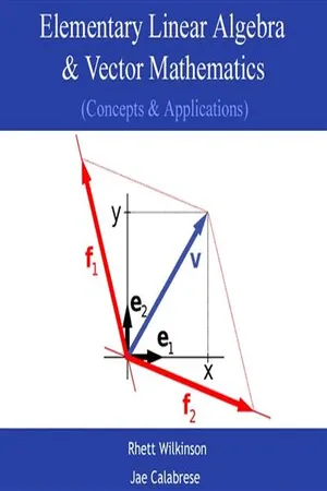
  Linear Algebra: Gateway to Mathematics

  Second Edition

  • Robert Messer(Author)
  • 2021(Publication Date)
  • American Mathematical Society

    (Publisher)

  5. Several other approaches to determinants are in common use. Here are two interesting alternatives. You should have little trouble finding references in your library if you prefer reading someone else’s exposition to embarking on your own discovery mission. Your goal is to use the alternative definition to derive the basic results of determinants. Be sure to weigh the advantages of not having to prove the properties used in the alternative definition against the work needed to derive the formula for the expansion of the determinant by minors. The results of Exercise 17 of Section 7.2 can be formulated in a more general setting. This leads to a definition of the determinant of an ? × ? matrix in terms of the ? -dimensional volume of the region in ℝ ? determined by the rows of the matrix. Some convention is needed regarding the sign of the determinant. Perhaps the most sophisticated approach is to define the determinant in terms of certain characteristic properties. As background information, you may first want to show that the determinant is the only function from 𝕄 ?,? to ℝ that is linear as a function of each of the ? rows, changes sign when two rows are interchanged, and maps the identity matrix to 1 . Hence, it is reasonable to take these three properties as a definition of the determinant. With this approach, the first order of business is to show that such a function does in fact exist and that it is unique. A clever way is to show that the set of all functions from 𝕄 ?,? to ℝ that satisfy the first two conditions is Project: Curve Fitting with Determinants 327 a one-dimensional subspace of 𝔽 𝕄 𝑛,𝑛 . Then all such functions are scalar multiples of the one that maps the identity matrix to 1 . Project: Curve Fitting with Determinants In Section 2.4 we saw how to use systems of linear equations to determine the coeffi-cients of a curve satisfying certain conditions.

  Sign up to read

  Learn more about book
• 

  eBook - PDF

  Matrices in Engineering Problems

  • Marvin Tobias(Author)
  • 2022(Publication Date)
  • Springer

    (Publisher)

  23 C H A P T E R 2 Determinants 2.1 INTRODUCTION The definition of a determinant is derived from the solution of linear algebraic equations. Since the single variable case is trivial, we will begin with the (2X2): a 11 x 1 + a 12 x 2 = c 1 a 21 x 1 + a 22 x 2 = c 2 . (2.1) To eliminate x 2 , we multiply the first equation by a 22 , and the second by a 12 , then subtract the second from the first: (a 11 a 22 − a 12 a 21 )x 1 = (a 22 c 1 − a 12 c 2 ) . (2.2) Equivalently, we may eliminate x 1 (by the same methods): (a 11 a 22 − a 12 a 21 )x 2 = (a 11 c 2 − a 21 c 1 ) . (2.3) The coefficients on both sides of (2.2) and (2.3) can be viewed as expansions via “cross-multiplication” of determinant arrays, as follows: ⎧ ⎪ ⎪ ⎪ ⎪ ⎪ ⎪ ⎪ ⎪ ⎪ ⎪ ⎪ ⎪ ⎪ ⎪ ⎨ ⎪ ⎪ ⎪ ⎪ ⎪ ⎪ ⎪ ⎪ ⎪ ⎪ ⎪ ⎪ ⎪ ⎪ ⎩ a 11 a 12 a 21 a 22 + - = (a 11 a 22 − a 12 a 21 ) a 11 c 1 a 21 c 2 + - = (a 11 c 2 − c 1 a 21 ) c 1 a 12 c 2 a 22 + - = (c 1 a 22 − a 12 c 2 ) (2.4) The square arrays in (2.4) “expand,” by the cross—multiplication indicated, to the scalars shown on the right sides. And, we define the determinant in terms of its expansion. Expansions are defined only for square arrays. The result of the expansion is a scalar expression, or numeric value. That is, the determinant is a scalar value. Further, from (2.2) and (2.3), the values of the variables are found as the ratio of these expanded determinants—all of which are known, given in the problem. 24 2. DETERMINANTS Three Variables: a 11 x 1 + a 12 x 2 + a 13 x 3 = c 1 a 21 x 1 + a 22 x 2 + a 23 x 3 = c 2 a 31 x 1 + a 32 x 2 + a 33 x 3 = c 3 .

  Sign up to read

  Learn more about book
• 

  eBook - PDF

  A Course of Mathematics for Engineerings and Scientists

  Volume 2

  • Brian H. Chirgwin, Charles Plumpton(Authors)
  • 2017(Publication Date)
  • Pergamon

    (Publisher)

  ( 0 ( i i ) ( i i i ) ( i v ) (v) 236 A COURSE OF MATHEMATICS 3:10 Linear dependence One of the 'elementary' operations we performed earlier on matrices con-sisted of adding multiples of different rows (or columns) to a given row (or column). This is briefly described as forming 'linear combinations' of rows. The determinant of a matrix is zero if one row (or column) is a linear combi-nation of other rows (or columns); in this case we say that the rows (or co-lumns) are 'linearly dependent'. This concept of linear dependence is very im-portant and occurs in many contexts. The use of the word 'linear' stems from the fact that the equation of a line in elementary analytical geometry is of the first degree in the current coordi-nates. A homogeneous linear relation y = f(x) between two variables x and y satisfies the following conditions: (i) f(cx) = cf(x) for arbitrary c and x; (ii) when y x = f{x x ) and y 2 = f(x 2 ) then y 1 +y 2 =/(*i+*2) for arbitrary xx and x 2 . This definition is generalised to a function u of many variables x, y, ..., z. The function u =/(x, y 9 ..., z) is a homogeneous linear function if it satisfies the following conditions : (i) f(cx, cy, ..., cz) = cf(x, y, ..., z) for arbitrary x, y, ..., z; (ii) when n x = f(x u y u ..., z x ) and u 2 = /(x 2 , j 2 , ..., z 2 ) then »i+w 2 = z f(x 1 +x2,yi+y2 9 ..., Z1+Z2). Accordingly a determinant is a linear function of the elements of any one row; the actual form of the relationship is given by the expansion in terms of cofactors If a set of quantities satisfies a relation of the form then (j) is a linear combination of 0 X , ... (j> k or $ is linearly dependent on the #!,..., k . Again, if we can find numbers k 19 A 2 ,... , not all zero, such that (3.63) we say that the <£, are linearly dependent on one another. Conversely, if we can- § 3 : 10] LINEAR EQUATIONS, MATRICES AND DETERMINANTS 237 not find any numbers A l5 ..., X k (except all of them zero) which satisfy eqn.

  Sign up to read

  Learn more about book
• 

  eBook - PDF

  An Introduction to Differential Equations

  Deterministic Modeling, Methods and Analysis(Volume 1)

  • Anil G Ladde, G S Ladde;;;(Authors)
  • 2012(Publication Date)
  • WSPC

    (Publisher)

  Chapter 1 Elements of Matrices, Determinants, and Calculus 1.1 Introduction This chapter serves as a review. It begins by highlighting a few ideas about the process of solving mathematics/education/research problems, and then covers rel-evant mathematical concepts and statements in linear algebra and the calculus of matrix functions. In particular, the algebra of matrices, the properties of deter-minants, some concepts about vector spaces, sets of independent and dependent vectors, methods for solving systems of linear-algebraic equations, and Wronskians of functions are discussed in Sections 1.3 and 1.4. Moreover, differential calculus of determinant functions, particularly a generalized mean-value theorem and Taylor’s formula for determinant functions, are developed in Section 1.5. These results play a very important role in finding solutions to linear differential equations, especially stochastic differential equations. Note that we are not attempting to teach linear algebra and multivariate calculus. This chapter not only serves as a reference guide for the reader, but it also is teaching guide for the instructor. 1.2 Problem-Solving Process One of the most important goals of education is to gain knowledge about the entire universe, and to apply it for the benefit of living things on the Earth. Its purpose is also to gain knowledge of the problem-solving process to eradicate or understand our ignorance. The presented knowledge about the problem-solving process can easily be applied in any area of science: biological, chemical, engineering, mathematical, medical, physical, political, social, etc. Currently, it is well recognized that the knowledge and practices employed in the mathematical-problem-solving processes provide a suitable background and the tools for solving problems arising in any discipline. In the 21st century, the question that is important to all of us is how to gain knowledge of the complex system (the 1

  Sign up to read

  Learn more about book
• 

  eBook - PDF

  Algebraic Number Theory for Beginners

  Following a Path From Euclid to Noether

  • John Stillwell(Author)
  • 2022(Publication Date)
  • Cambridge University Press

    (Publisher)

  7 Determinant Theory Preview The determinant function is a concept of linear algebra frequently skimmed over or minimized in modern treatments of the subject. At the same time, books on algebraic number theory tend to assume sophisticated properties of the determinant – such as its relationship to trace, norm, and characteristic polynomial – to be already known from a basic linear algebra course. Under these circumstances it seems useful to develop the determinant concept from scratch and then transition to its applications in algebraic number fields. This is what we aim to do in this chapter, hopefully making the book more self-contained without greatly increasing its size. We begin with an elementary treatment of determinants, due to Artin (1942). His approach leads rapidly to methods for evaluating determinants, applications to linear equations, and to the all-important multiplicative property. We can then prove the invariance of the determinant under change of basis and deduce the basis-independence of trace, norm, and characteristic polynomial. This leads in turn to relations between the trace and norm of an algebraic number and the roots of its minimal polynomial. With these foundations we can then introduce the discriminant, which tests whether an n-tuple of members of a field F of degree n over Q is a basis for F . This paves the way for the study of integral bases in the next chapter. These generalize the concept of basis from vector spaces to certain kinds of modules, such as the algebraic number rings Z E . 149 150 7 Determinant Theory Figure 7.1 Emil Artin (1898–1962) (used with permission of Tom Artin and his siblings). 7.1 Axioms for the Determinant There are many ways to define the determinant function and derive its basic properties, none of them completely straightforward. One that is elementary, yet algebraic in spirit, is given in Artin (1942), pages 12–20.

  Sign up to read

  Learn more about book
• 

  eBook - PDF

  Precalculus with Limits

  • Ron Larson(Author)
  • 2021(Publication Date)
  • Cengage Learning EMEA

    (Publisher)

  Copyright 2022 Cengage Learning. All Rights Reserved. May not be copied, scanned, or duplicated, in whole or in part. Due to electronic rights, some third party content may be suppressed from the eBook and/or eChapter(s). Editorial review has deemed that any suppressed content does not materially affect the overall learning experience. Cengage Learning reserves the right to remove additional content at any time if subsequent rights restrictions require it. 560 Chapter 8 Matrices and Determinants GO DIGITAL EXAMPLE 10 Squaring a Matrix Find A 2 , where A = [ 3 -1 1 2 ] . (Note: A 2 = AA.) Solution A 2 = [ 3 -1 1 2 ][ 3 -1 1 2 ] = [ 8 -5 5 3 ] Checkpoint Audio-video solution in English & Spanish at LarsonPrecalculus.com Find A 2 , where A = [ 2 3 1 -2 ] . If A is an n × n matrix, then the identity matrix has the property that AI n = A and I n A = A. For example, [ 3 1 -1 -2 0 2 5 4 -3 ][ 1 0 0 0 1 0 0 0 1 ] = [ 3 1 -1 -2 0 2 5 4 -3 ] AI = A and [ 1 0 0 0 1 0 0 0 1 ][ 3 1 -1 -2 0 2 5 4 -3 ] = [ 3 1 -1 -2 0 2 5 4 -3 ] . IA = A Properties of Matrix Multiplication Let A, B, and C be matrices and let c be a scalar. 1. A(BC) = (AB)C Associative Property of Matrix Multiplication 2. A(B + C) = AB + AC Left Distributive Property 3. (A + B)C = AC + BC Right Distributive Property 4. c(AB) = (cA)B = A(cB) Associative Property of Scalar Multiplication Definition of the Identity Matrix The n × n matrix that consists of 1’s on its main diagonal and 0’s elsewhere is called the identity matrix of dimension n × n and is denoted by I n = [ 1 0 0  0 0 1 0  0 0 0 1  0 . . . . . . . . . . . . 0 0 0  1 ] . Identity matrix Note that an identity matrix must be square. When the dimension is understood to be n × n, you can denote I n simply by I. Copyright 2022 Cengage Learning. All Rights Reserved. May not be copied, scanned, or duplicated, in whole or in part. Due to electronic rights, some third party content may be suppressed from the eBook and/or eChapter(s).

  Sign up to read

  Learn more about book
• 

  eBook - PDF

  Algebra & Trig

  • Ron Larson(Author)
  • 2021(Publication Date)
  • Cengage Learning EMEA

    (Publisher)

  Copyright 2022 Cengage Learning. All Rights Reserved. May not be copied, scanned, or duplicated, in whole or in part. Due to electronic rights, some third party content may be suppressed from the eBook and/or eChapter(s). Editorial review has deemed that any suppressed content does not materially affect the overall learning experience. Cengage Learning reserves the right to remove additional content at any time if subsequent rights restrictions require it. 720 Chapter 10 Matrices and Determinants GO DIGITAL EXAMPLE 10 Squaring a Matrix Find A 2 , where A = [ 3 -1 1 2 ] . (Note: A 2 = AA.) Solution A 2 = [ 3 -1 1 2 ][ 3 -1 1 2 ] = [ 8 -5 5 3 ] Checkpoint Audio-video solution in English & Spanish at LarsonPrecalculus.com Find A 2 , where A = [ 2 3 1 -2 ] . If A is an n × n matrix, then the identity matrix has the property that AI n = A and I n A = A. For example, [ 3 1 -1 -2 0 2 5 4 -3 ][ 1 0 0 0 1 0 0 0 1 ] = [ 3 1 -1 -2 0 2 5 4 -3 ] AI = A and [ 1 0 0 0 1 0 0 0 1 ][ 3 1 -1 -2 0 2 5 4 -3 ] = [ 3 1 -1 -2 0 2 5 4 -3 ] . IA = A Properties of Matrix Multiplication Let A, B, and C be matrices and let c be a scalar. 1. A(BC) = (AB)C Associative Property of Matrix Multiplication 2. A(B + C) = AB + AC Left Distributive Property 3. (A + B)C = AC + BC Right Distributive Property 4. c(AB) = (cA)B = A(cB) Associative Property of Scalar Multiplication Definition of the Identity Matrix The n × n matrix that consists of 1’s on its main diagonal and 0’s elsewhere is called the identity matrix of dimension n × n and is denoted by I n = [ 1 0 0  0 0 1 0  0 0 0 1  0 . . . . . . . . . . . . 0 0 0  1 ] . Identity matrix Note that an identity matrix must be square. When the dimension is understood to be n × n, you can denote I n simply by I. Copyright 2022 Cengage Learning. All Rights Reserved. May not be copied, scanned, or duplicated, in whole or in part. Due to electronic rights, some third party content may be suppressed from the eBook and/or eChapter(s).

  Sign up to read

  Learn more about book
• 

  eBook - PDF

  Elementary Linear Algebra, International Metric Edition

  • Ron Larson(Author)
  • 2017(Publication Date)
  • Cengage Learning EMEA

    (Publisher)

  To find the determinant of A T = bracketleft.alt2 3 1 -2 2 0 0 -4 -1 5 bracketright.alt2 expand by cofactors in the second column to obtain uni2223 A T uni2223 = 2 ( -1 ) 3 uni2223 1 -2 -1 5 uni2223 = ( 2 )( -1 )( 3 ) = -6. THEOREM 3.9 Determinant of a Transpose If A is a square matrix, then det ( A ) = det ( A T ) . William Perugini/Shutterstock.com LINEAR ALGEBRA APPLIED Systems of linear differential equations often arise in engineering and control theory. For a function f ( t ) that is defined for all positive values of t , the Laplace transform of f ( t ) is F ( s ) = integral.alt1 ∞ 0 e -st f ( t ) dt provided that the improper integral exists. Laplace transforms and Cramer’s Rule, which uses determinants to solve a system of linear equations, can sometimes be used to solve a system of differential equations. You will study Cramer’s Rule in the next section. Copyright 2018 Cengage Learning. All Rights Reserved. May not be copied, scanned, or duplicated, in whole or in part. WCN 02-300 3.3 Exercises 131 3.3 Exercises See CalcChat.com for worked-out solutions to odd-numbered exercises. The Determinant of a Matrix Product In Exercises 1–6, find (a) uni2223 A uni2223 , (b) uni2223 B uni2223 , (c) AB , and (d) uni2223 AB uni2223 . Then verify that uni2223 A uni2223uni2223 B uni2223 equal.bold uni2223 AB uni2223 . 1. A = bracketleft.alt2 -2 4 1 -2 bracketright.alt2 , B = bracketleft.alt2 1 0 1 -1 bracketright.alt2 2. A = bracketleft.alt2 3 4 4 3 bracketright.alt2 , B = bracketleft.alt2 2 5 -1 0 bracketright.alt2 3. A = bracketleft.alt2 -1 1 0 2 0 1 1 1 0 bracketright.alt2 , B = bracketleft.alt2 -1 0 0 0 2 0 0 0 3 bracketright.alt2 4. A = bracketleft.alt2 2 1 3 0 -1 1 1 2 0 bracketright.alt2 , B = bracketleft.alt2 2 0 3 -1 1 -2 4 3 1 bracketright.alt2 5. A = bracketleft.alt2 2 1 2 1 0 -1 3 2 1 0 1 3 1 1 0 0 bracketright.alt2 , B = bracketleft.alt2 1 2 1 3 0 1 1 2 -1 0 -1 1 1 2 0 0 bracketright.alt2 6.

  Sign up to read

  Learn more about book