Mean Value Theorem for Integrals

5 Key excerpts on "Mean Value Theorem for Integrals"

• 

  eBook - ePub

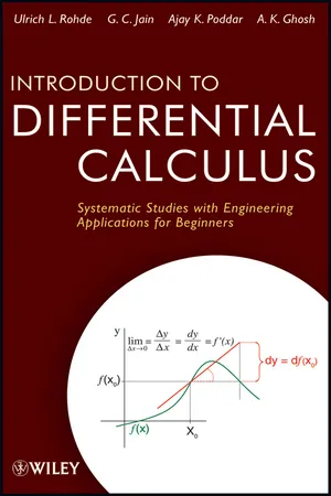
  Introduction to Differential Calculus

  Systematic Studies with Engineering Applications for Beginners

  • Ulrich L. Rohde, G. C. Jain, Ajay K. Poddar, A. K. Ghosh(Authors)
  • 2012(Publication Date)
  • Wiley

    (Publisher)

  4

  The conclusions of the MVT are intuitively appealing and its hypotheses are naturally expected. Further, its applications will be found marvelously tangible (i.e., fitting with experience). The student will find in the MVT, an ever present tool just waiting to be applied, both in proving theorems and in solving problems.

  The adjective “mean ” carries both the notions “between ” and “average ”, each of which gives a significant clue to the basic idea in the theorem. What the MVT does, is single out a derivative value that plays the role of an average derivative value, and this derivative value is attained at a point strictly between the end points of the interval domain of the function.

  Consider a continuous function ,

  which is differentiable at every point of the open interval (a , b ).5

  Figure 20.12

  What the MVT does is to identify the difference quotient with the derivative f ′(x ) evaluated at a point (say) c , lying strictly between a and b .

  That is,

  It must be clearly understood once and for all that the location of c is not really pinpointed ; we only know that it lies somewhere inside an open interval (a , b ). But, the interesting fact is the mere knowledge that c is a mean point (i.e., it lies strictly between the end points of the interval) shows the real power behind the theorem and its applications . Of course, the exact location of c can be found in some cases (as we have seen in some solved examples) but in general, it is never needed in any application.

  Many important concepts in mathematics are based on Existence Theorems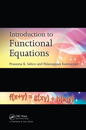

  Sign up to read

  Learn more about book
• 

  eBook - PDF

  Introduction to Functional Equations

  • Prasanna K. Sahoo, Palaniappan Kannappan(Authors)
  • 2011(Publication Date)
  • Chapman and Hall/CRC

    (Publisher)

  Chapter 16 Mean Value Type Functional Equations 16.1 Introduction In this chapter, we will examine some functional equations that arise from the Lagrange mean value theorem. We call these functional equa-tions the mean value type of functional equations. The study of this type of functional equations was started by Acz´ el (1985), Haruki (1979) and Kuczma (1991a, 1991b). A detailed account on mean value type func-tional equations can be found in the book Mean Value Theorems and Functional Equations by Sahoo and Riedel (1998). 16.2 The Mean Value Theorem The mean value theorem (MVT) whose proof can be in the book Mean Value Theorems and Functional Equations by Sahoo and Riedel (1998) (see pages 25–27) is the following. Theorem 16.1. Suppose the real-valued function f is continuous on the closed interval [ a, b ] and is differentiable on the open interval ( a, b ) . Then there exists η ∈ ( a, b ) such that f 0 ( η ) = f ( b ) -f ( a ) b -a . (16.1) The equation of the tangent line at the point ( η, f ( η )) is given by y = ( x -η ) f 0 ( η ) + f ( η ) . (16.2) The equation of the secant line joining the points ( a, f ( a )) and ( b, f ( b )) 243 244 Introduction to Functional Equations is given by y = ( x -a ) f ( b ) -f ( a ) b -a + f ( a ) . (16.3) If the secant line is parallel to the tangent line at η (see Figure 16.1), then f 0 ( η ) = f ( b ) -f ( a ) b -a . (16.4) -6 y 0 x tangent line secant line a η b . . . . . . . . . . . . . . . . . . . . . f ( x ) Figure 16.1. Geometrical interpretation of MVT. This Lagrange’s mean value theorem is an important theorem in differentiable calculus. This theorem was first discovered by Joseph Louis Lagrange (1736–1813), but the idea of applying the Rolle’s theorem to a suitably contrived auxiliary function was given by Ossian Bonnet (1819– 1892). However, the first statement of the theorem appears in a paper by renowned physicist Andr´ e-Marie Amp´ ere (1775–1836).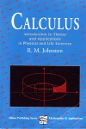

  Sign up to read

  Learn more about book
• 

  eBook - PDF

  Calculus

  Introductory Theory and Applications in Physical and Life Science

  • R. M. Johnson(Author)
  • 1995(Publication Date)
  • Woodhead Publishing

    (Publisher)

  11 Further Applications of Integration 11.1 INTRODUCTION In Chapter 5, integration was applied to the calculation of areas and volumes. A number of additional applications are considered in this chapter and in each case Theorem 5.1 (fundamental theorem of integral calculus) is applied. As in Chapter 5, the formal procedure of the theorem will be relaxed where appropriate by writing a differential instead of Δχ for the strip width and using the integral sign to denote summation. 11.2 THE MEAN VALUE OF A FUNCTION Consider the function y = fix) in the interval a < x < b. Divide the interval into n sub-intervals of width Δχ, i.e. n Ax = b—a. The ordinates^o.Ji.^2 )>n are as shown in Fig. 11.1. The average value of y in a < x < b is approximately n Σ yi*x JO +y +yi + ■■■+y n »=<> n+ 1 (b-a) + Ax ' since b-a n = . Δχ We define the mean value of y, denoted by y, as the limit of this summation as Ax -»■ 0. Using Theorem 5.1, we have 242 Further Applications of Integration [Ch. 11 y =/(*) y=-I ydx. h — n n When dealing with periodic functions a useful parameter is the root-mean-square (RMS) value. For a function/(f) of period Tthe RMS value is defined as J 7i>» ,d '· i.e. the square root of the mean value of the function squared taken over an interval equal to one period. Example 11.1 (i) Find the mean value of the function* 2 + 1 in the interval 1 < x < 3. (ii) Find the RMS value of a 50 Hz voltage signal of amplitude 250 V. (i) Let.y=;c 2 + 1. àx 1 T X — + x 3 16 = T · (ii) The frequency of 50 Hz is 50 X 2ττ = ΙΟΟτ rad/s, i.e. V= 250 sin ΙΟΟπί and the period Tis 1/50 s. Therefore, Sec. 11.2] The Mean Value of a Function 243 1 r o.o2 mean square value = | 250 sin· 4 lOOntdt 0.02 J o r o.o2 250 2 = 50 J (1 - cos 200πί) dt •Ό 2 = 25 X 250 2 1 20Ο7Γ sin 200« 0.02 = 25 X 250 2 X 0.02 = 0.5 X 250 2 . RMS value = V0.5 X 250 2 250 Problems 1. Find the mean value of the following functions. (0 y = 1 +x 2 • K I < 1 . (ii) v = sin It, 0 < t < - .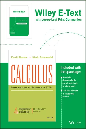

  Sign up to read

  Learn more about book
• 

  eBook - PDF

  Calculus

  Resequenced for Students in STEM

  • David Dwyer, Mark Gruenwald(Authors)
  • 2017(Publication Date)
  • Wiley

    (Publisher)

  (Hint: Consider the function f (x) = sin 2x on the interval [s, t] and follow the lead of Example 5.) 38. Use the MVT to show that √ 1 + t ≤ t 2 + 1 for t ≥ 0. (Hint: Apply the MVT to the function f (x) = √ 1 + x on the interval [0, t].) 39. Let f (x) = |x|. a) Find the average rate of change of f on [-1, 2]. b) Show that there is no number c on (-1, 2) for which f 0 (c) is equal to the average rate of change found in part a. c) Does the answer to part b contradict the Mean Value Theorem? Explain. 40. Let f (x) = x 2 3 . a) Find f 0 (x). b) Does f satisfy the conditions for the Mean Value Theorem on the interval (-1, 27)? c) Find a number c in (-1, 27) such that the instanta- neous rate of change of f at c is equal to the average rate of change of f on (-1, 27). d) Does your answer to part c contradict the Mean Value Theorem? Explain. Applications 41. Velocity A ball thrown up into the air has height in feet after t seconds given by s(t) = -16t 2 + 32t + 5. a) Find the average velocity of the ball from t = 1 to t = 2. b) Find the time at which the instantaneous velocity of the ball is the same as the average velocity found in part a. 42. Water Flow During a 3-minute time interval, the flow of water into a tank is regulated in such a way that the volume after t minutes is V (t) = 0.1t 3 + 2t + 5 gallons. a) Find the average rate of flow of the water over the 3-minute time interval. b) Find the time at which the instantaneous flow rate of the water is the same as the average rate of flow found in part a. 43. Marginal and Average Costs In economics, C(x) repre- sents the cost of producing x units, C(x) = C(x) x is the average cost per unit, and C 0 (x) is the marginal cost.

  Sign up to read

  Learn more about book
• 

  eBook - PDF

  The Fundamentals of Mathematical Analysis

  • G. M. Fikhtengol'ts, I. N. Sneddon(Authors)
  • 2014(Publication Date)
  • Pergamon

    (Publisher)

  CHAPTER 6 BASIC THEOREMS OF DIFFERENTIAL CALCULUS § 1. Mean value theorems ___ 100. Fermat's theorem. The knowledge of the derivative (or a number of derivatives) of a function makes it possible to draw conclusions regarding the function itself. The basis of various appli-cations of the concept of a derivative (see Chapters 7 and 13) rests on certain simple but important theorems and formulae to which this chapter is devoted. We begin by examining a statement which is linked with the name of Fermât 1 . Of course, he did not announce it in the form in which we present it here (Fermât did not know of the concept of a de-rivative); however, our form re-establishes the essence of Fermafs device as applied by him to determining the greatest and the smallest values of a function (see Chapter 14). FERMAT'S THEOREM. Suppose that a function f(x) is defined in an interval 9C and that it takes at an interior point of the interval its greatest (smallest) value. If at this point there exists the finite derivative f '(c), then, necessarily, f (c) = 0. Proof For definiteness let f(x) take at a point c its greatest value; hence for all x from 9C we have f(*)c the expression X — C and hence passing to the limit, x-»c + 0, we obtain /'(c)<0. (1) If now x < c, then x—c passing to the limit, x->c — 0, we have fc) = 0. (2) Comparing relations (1) and (2) we arrive at the required result /'(c) = 0. Remark. The reasoning carried out above proves, essentially, that at the considered point c an infinite (two-sided) derivative cannot exist.

  Sign up to read

  Learn more about book