Radial Distribution Function

4 Key excerpts on "Radial Distribution Function"

• 

  eBook - PDF

  Advances in Chemical Physics, Volume 34

  • Ilya Prigogine, Stuart A. Rice(Authors)
  • 2009(Publication Date)
  • Wiley-Interscience

    (Publisher)

  These forms all give the same treat- ment of the data, with various constants being incorporated into the nor- malization of the experimental I(s). All the studies of molecular systems reviewed in this paper make use.ofone form or another of (2.21). Interpretation of the ERDF' in terms of the individual atomic pair dis- tributions has been discussed by Warren,'20 M e n ~ l e l , ~ ~ Waser and Scho- maker,'22 and Pings and W a ~ e r . ' ~ As is the case with the previously dis- cussed Fourier transforms, the kernel of (2.21) is sometimes modified by an artificial temperature factor of the form'22 e-bs2 (see Refs. 37, 44, 105); and the ERDF' can be interpreted in terms of ideal peaks'22 (see also Refs. 37,44). Since the ERDF' contains information about the intramolecular as well as the intermolecular structure, it is possible to infer molecular parameters from the ERDF'. This can be done by either assuming the molecular model 176 J. F. KARNICKY AND C. J. PINGS and obtaining the parameters by fitting to the ERDF (see Refs, 37, 44, 82, 85,105) or by determining the molecular model itself by fitting to the ERDF' (see Refs. 60, 123). Once the molecular structure is known, it is possible to subtract the scattering due to the intramolecular structure from Z(s) and infer properties of the intermolecular structure from the ERDF' (see Ref. 82) Molecular Radial Distribution Functions. Equation (2.19) has been used by many researchers to calculate the radial distribution of heteronuclear molecules in a fluid. The principal differencein the various methods lies in the calculation of the scattering factor for the molecule, F2(s). The most frequently used approximation to F2(s) is the spherically aver- aged value for the sums of the atomic scattering factors in the m o l e c ~ l e : ~ ~ , ' ~ L(s)A(s) sin rijs F2(s) = C i, j rijs (2.27) where rij is the distance between atoms i andj in the molecule.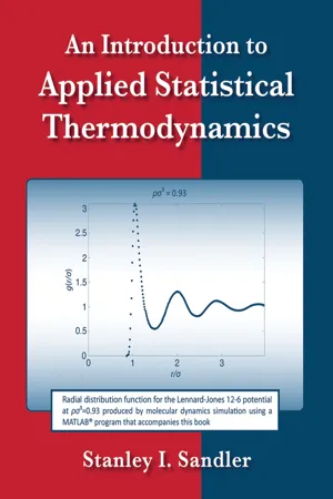

  Sign up to read

  Learn more about book
• 

  eBook - PDF

  An Introduction to Applied Statistical Thermodynamics

  • Stanley I. Sandler(Author)
  • 2015(Publication Date)
  • Wiley

    (Publisher)

  For molecules with more atoms, the number of different correlation functions increases. A second method of determining the Radial Distribution Function is by use of statis- tical mechanical theory, and there are several ways to proceed. One method has been to use the assumption of pairwise additivity of the potential and the graph theory of clusters, as was done in the development of expressions for the virial coefficients from the canonical ensemble, to develop integral equations for the Radial Distribution Function. The graph theory development is extremely complicated, so approximations are made leading to models with names such as the Percus-Yevick, hypernetted chain, 198 Chapter 11: Interacting Molecules in a Dense Fluid. Configurational Distribution Functions g H g ClCl g HCl Figure 11.4-1 Atom-atom correlation functions for the two-center HCl molecule. and mean spherical approximations, as examples. Some of these will be discussed in the Chapter 12. Such integral equations are usually solved numerically to obtain the Radial Distribution Function at various temperatures and densities. However, after numerical evaluation, one only has a table of numbers and not analytic expressions for the Radial Distribution Function as a function of separation distance, temperature, and density for the model pairwise-additive potential obtained from an approximate theory, and not an analytic expression. A third method of obtaining the Radial Distribution Function is by molecular-level computer simulation, which is discussed in some detail in Chapter 13. A brief intro- duction, for the sake of continuity, is given here. In this method, by computer programming, molecules are described by model potentials (usually, but not always, pairwise additive) and are considered to be in a box that exists in the memory of a computer.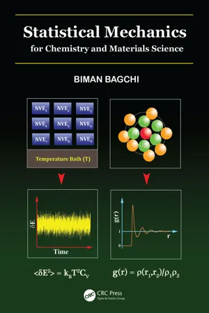

  Sign up to read

  Learn more about book
• 

  eBook - ePub

  Statistical Mechanics for Chemistry and Materials Science

  • Biman Bagchi(Author)
  • 2018(Publication Date)
  • CRC Press

    (Publisher)

  get ρ (1) (r) = N ∫ d r 2 d r 3 … d r N e − β U N V ∫ d r 2 d r 3 … d r N e − β U N = ρ 11.11 11.11 The above analysis suggests a useful normalized representation of distribution functions. We now consider two-particle distribution and suppose that we have fixed the position of two particles at r 1 and r 2. If there is no interaction between the particles, then the joint probability density will. be ρ N (2) (r 1, r 2) = N ! (N − 2) ! ∫ d r 3 d r 4 d r 5 … ∫ d r N e − β U N (r N) Z N, ρ N (2) (r 1, r 2) = N (N − 1) V 2. V 2 Z N. ∫ d r 3 d r 4[--=PLGO-SEP. ARATOR=--]d r 5 … ∫ d r N e − β U N (r N) 11.12 11.12 Now in the absence of any intermolecular interaction and any external potential, Eq. (11.12) leads to the decomposition of two-particle density in terms of two single particle distributions ρ N (2) (r 1, r 2) = N (N − 1) V N − 2 V N = N (N − 1) V 2 = ρ 2 11.13 11.13 So the joint probability density can be factorized in the ideal case. But in a system where interaction is present it cannot be simply factorized. We now define a dimensionless measure of the two particle distribution function, popularly known as the Radial Distribution Function (RDF) as follows g (r) = ρ N (2) (r 1, r 2) ρ 2 = V 2 Z N. ∫ d r 3 d r 4 d r 5 … ∫ d r N e − β U N (r N) 11.14 11.14 Radial Distribution Function (RDF) thus defined provides a useful measure of the deviation from a completely random arrangement of its molecules. For example, in dense liquids, it provides a quantitative measure of the short range order (SRO) of the liquid. This short range order determines many of the properties of the liquid, including its freezing condition, and also dynamical properties, like diffusion constant. Also note the limiting behavior. When the mutual separation between particles tends to infinity, correlation between positions of particles goes to zero and g N (n) (r n) → 1. Eq

  Sign up to read

  Learn more about book
• 

  eBook - ePub

  Underneath the Bragg Peaks

  Structural Analysis of Complex Materials

  • Takeshi Egami, Simon J.L. Billinge(Authors)
  • 2012(Publication Date)
  • Pergamon

    (Publisher)

  c ).

  There is one final feature of G (r ), again related to its experimental importance. In a real experiment, S (Q ) is measured only over a finite range of Q . The consequence in the Fourier transform is that termination ripples appear; ripples with a wavelength ∼ 2π /Q max . Mathematically, this comes about because the theoretical G (r ) becomes convoluted with the Fourier transform of the termination function. This is discussed in more detail in Section 3.5 . For completeness, we simply make the point that it is G (r ) that should be thus convoluted, not ρ (r ) or g (r ).

  3.1.3.3 The Radial Distribution Function, R (r )

  The next-correlation function we discuss is the most physically intuitive. The PDF, g (r ), is related to the RDF, R (r ), by

  (3.37)

  The RDF has the useful property that the quantity R (r )dr gives the number of atoms in an annulus of thickness dr at distance r from another atom. For example, the coordination number, or the number of neighbors, N C , is given by

  (3.38)

  where r 1 and r 2 define the RDF peak corresponding to the coordination shell in question. This suggests a scheme for calculating PDFs from atomic models. Consider a model consisting of a large number of atoms situated at positions r ν with respect to some origin. Expressed mathematically, this amounts to a series of delta functions, δ (r  − r ν ). The RDF is then given as

  (3.39)

  Here, the b values are the atomic scattering lengths of the ions and the sums are over every atom in the sample. This is a restatement of Eq. (1.1) , and indeed, this property of R (r ) is the origin of that equation. In the case of X-rays, the b values are replaced by f ν (0), the value of the atomic scattering factor for the ν th atom at Q  = 0. Note that f ν (0) ∼ Z ν , the atomic number of the species. The value r νμ  = |r ν  − r μ | is the magnitude of the separation of the ν th and μ

  Sign up to read

  Learn more about book