Boundary Layer

6 Key excerpts on "Boundary Layer"

• 

  No longer available |Learn more

  Aerodynamics & its Applications

  • (Author)
  • 2014(Publication Date)
  • Learning Press

    (Publisher)

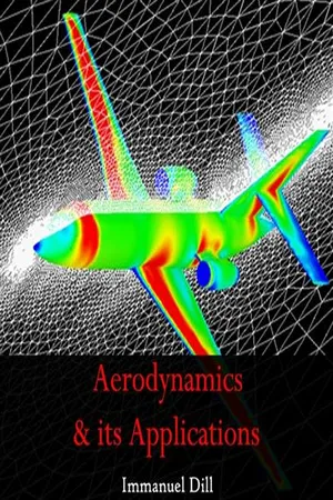
  ____________________ WORLD TECHNOLOGIES ____________________ Chapter 5 Boundary Layer & Turbulence Boundary Layer Boundary Layer visualization, showing transition from laminar to turbulent condition In physics and fluid mechanics, a Boundary Layer is that layer of fluid in the immediate vicinity of a bounding surface where effects of viscosity of the fluid are considered in detail. In the Earth's atmosphere, the planetary Boundary Layer is the air layer near the ground affected by diurnal heat, moisture or momentum transfer to or from the surface. On an aircraft wing the Boundary Layer is the part of the flow close to the wing. The Boundary Layer effect occurs at the field region in which all changes occur in the flow pattern. The Boundary Layer distorts surrounding non-viscous flow. It is a phenomenon of viscous forces. This effect is related to the Reynolds number. Laminar Boundary Layers come in various forms and can be loosely classified according to their structure and the circumstances under which they are created. The thin shear layer which develops on an oscillating body is an example of a Stokes Boundary Layer, whilst the Blasius Boundary Layer refers to the well-known similarity solution for the steady Boundary Layer attached to a flat plate held in an oncoming unidirectional flow. When a fluid rotates, viscous forces may be balanced by the Coriolis effect, rather than convec- ____________________ WORLD TECHNOLOGIES ____________________ tive inertia, leading to the formation of an Ekman layer. Thermal Boundary Layers also exist in heat transfer. Multiple types of Boundary Layers can coexist near a surface simultaneously. Aerodynamics The aerodynamic Boundary Layer was first defined by Ludwig Prandtl in a paper presented on August 12, 1904 at the third International Congress of Mathematicians in Heidelberg, Germany.

  Sign up to read

  Learn more about book
• 

  eBook - ePub

  Coulson and Richardson's Chemical Engineering

  Volume 1B: Heat and Mass Transfer: Fundamentals and Applications

  • R. P. Chhabra, V. Shankar(Authors)
  • 2017(Publication Date)
  • Butterworth-Heinemann

    (Publisher)

  Chapter 3

  The Boundary Layer

  Abstract

  When a fluid flows over a surface, the part of the stream that is close to the surface suffers a significant retardation, and a velocity profile is developed in the fluid. The velocity gradients are higher at the surface and progressively smaller with distance from the surface. The thickness of the Boundary Layer (a layer close to the surface in which the velocity increases from zero at the surface to a near-constant stream velocity at its outer boundary) may be arbitrarily defined as the distance from the surface at which the velocity reaches some proportion (such as 0.9, 0.99, and 0.999) of the undisturbed stream velocity. Alternatively, it is possible to approximate thickness to the velocity profile by means of an equation which gives the distance from the surface at which the velocity gradient is zero and the velocity is equal to the stream velocity. The flow conditions in the Boundary Layer are of considerable interest to chemical engineers because these influence not only the drag effect of the fluid on the surface but also the heat or mass transfer rates where a temperature or a concentration gradient exists. In this chapter, we will discuss the concept of velocity Boundary Layer, thermal Boundary Layer and concentration Boundary Layer.

  Keywords

  Boundary Layer; Velocity; Heat transfer; Streamline flow; Mass transfer; Momentum equation

  3.1 Introduction

  When a fluid flows over a solid surface, that part of the stream that is close to the surface suffers a significant retardation owing to the no-slip boundary condition at the fluid-solid boundary, and thus a velocity profile develops in the fluid. The velocity gradients are steepest close to the surface and become progressively smaller with distance from the surface. Although theoretically there is no outer limit at which the velocity gradient becomes zero, it is convenient to divide the flow into two parts for practical purposes:

  Sign up to read

  Learn more about book
• 

  Available until 4 Dec |Learn more

  Fluid Mechanics

  An Intermediate Approach

  • Bijay Sultanian(Author)
  • 2015(Publication Date)
  • CRC Press

    (Publisher)

  349 8 Boundary Layer Flow 8.1 Introduction Because of the nonzero viscosity of real fluids, all flows feature the no-slip condition at a solid boundary, resulting in a Boundary Layer flow with high transverse velocity gradients and wall shear stress. The effect of viscosity is predominantly confined to the bound-ary layers. Outside the Boundary Layer, the effect of viscosity may be considered negli-gible and the flow modeled as a potential flow, discussed in Chapter 6. Anderson (2005) captures the groundbreaking role of Ludwig Prandtl in first presenting the concept of the Boundary Layer in 1904 to the Mathematical Congress in Heidelberg, Germany, in an article titled, “On the Fluid Motion with Very Little Viscosity.” In his 10-minute presenta-tion on the subject, Prandtl revolutionized the understanding and analysis of fluid flows of great engineering interest. The idea of a thin Boundary Layer at the surface of a body in fluid flow explains the mechanism of separation under an adverse pressure gradient in the flow direction. If we had today’s computing power to numerically solve the complete set of Navier–Stokes equations, we would have perhaps missed the development of the bound-ary layer theory and the simplifications it brings in solving many engineering problems involving fluid flow, including heat and mass transfer. The drag force acting on a body consists of two parts: (1) frictional drag—due to the inte-grated effect of the shear stress distribution along the surface of the body—and (2) form drag—due to the integrated effect of the pressure distribution normal to the surface of the body. When the Boundary Layer separates, it creates a wake region of lower pressure behind the body, significantly increasing the form drag, which could be higher than the frictional drag on a bluff body.

  Sign up to read

  Learn more about book
• 

  eBook - ePub

  Fluid Mechanics, Hydraulics, Hydrology and Water Resources for Civil Engineers

  • Amithirigala Widhanelage Jayawardena(Author)
  • 2021(Publication Date)
  • CRC Press

    (Publisher)

  Chapter 7 Viscous fluid flow – Boundary Layer

  7.1 Introduction

  Fluids, in general, can be classified as ideal fluids and viscous or real fluids. Ideal fluids are assumed to have no viscosity although all fluids, in reality, have some viscosity. The viscous effect in fluid flow is confined to a thin layer near the boundary of flow, which is known as the Boundary Layer. Outside the region of the Boundary Layer, the fluid is assumed to be ideal, and the flow is sometimes referred to as potential flow. The general concept of Boundary Layer was introduced by Prandtl in 1904. It is an important and significant concept in Fluid Mechanics and provides a useful link between ideal fluids and real fluids. For fluids having relatively small viscosity, the effect of internal friction in a fluid is appreciable only in a narrow region surrounding the fluid boundaries.

  In the case of a flat plate placed in a flow field, the velocity (relative to the boundary) of the fluid at the boundary is zero. This is called the no-slip boundary condition. The flow velocity across the flow, therefore, varies from zero to its full value with a steep velocity gradient. Because of the viscosity of the fluid, this velocity gradient gives rise to shear stresses, which retard the flow flowing near the boundary. The region affected is called the Boundary Layer , or friction layer.

  The velocity in the boundary-layer approaches the velocity in the main flow asymptotically. The Boundary Layer is very thin at the upstream end of a streamlined body at rest in an otherwise uniform flow. As the layer moves downstream, the continual action of shear stress tends to slow down additional fluid particles causing the thickness of the Boundary Layer to increase in the downstream direction.

  For smooth upstream boundaries, the Boundary Layer starts as laminar . As the thickness increases, the flow becomes turbulent and transforms into turbulent Boundary Layer . The point at which the transition from laminar to turbulent depends upon the roughness of the surface, the turbulence in the mainstream, the pressure gradient in the mainstream just outside the Boundary Layer and the local Reynolds number. Even within the turbulent Boundary Layer, there exists a very thin layer close to the boundary where the viscous effects are significant. This is called the laminar sub-layer,

  Sign up to read

  Learn more about book
• 

  eBook - PDF

  Physics of Continuous Matter

  Exotic and Everyday Phenomena in the Macroscopic World

  • B. Lautrup(Author)
  • 2011(Publication Date)
  • CRC Press

    (Publisher)

  28 Boundary Layers At large Reynolds number, a fluid will behave as ideal nearly everywhere, except close to solid boundaries where the no-slip condition requires the speed of the fluid to match the speed of the boundary wall. Here, transition layers will arise in which the velocity of the flow changes quickly from the velocity of the wall to the velocity in the fluid at large. Boundary Layers are typically thin compared to the radii of curvature of the solid walls. Ludwig Prandtl (1875–1953). German physicist, often called the father of aerodynamics. De-veloped Boundary Layer theory, and contributed to wing the-ory, streamlining, compressible subsonic airflow, and turbulence [And05, O’M10]. (Source: Wiki-media Commons.) In a Boundary Layer the character of the flow thus changes from creeping near the boundary to ideal well outside. It is a general trait that the most interesting physics takes place in such transition regions. Humans, living out their lives in nearly ideal flows of air and water at Reynolds numbers in the millions with Boundary Layers only millimeters thick, are normally not conscious of them. Smaller animals eking out an existence at the surface of a stone in a river may be much more aware of the vagaries of Boundary Layer physics, which may even influence their body shapes and internal layout of organs. Boundary Layers serve to “insulate” bodies from the ideal flow that surrounds them. They have a “life of their own” and may separate from the solid walls and wander into regions containing only fluid. Detached layers may again split up, creating complicated unsteady turbulent patterns of whirls and eddies. Systematic Boundary Layer theory was initiated by Prandtl in 1904 and has in the twentieth century become a major subtopic of fluid mechanics. Advanced understanding of fluid mechanics begins with an understanding of Boundary Layers, although there is still no simple theory capable of predicting where separation takes place.

  Sign up to read

  Learn more about book
• 

  eBook - PDF

  Sir James Lighthill And Modern Fluid Mechanics

  • Lokenath Debnath(Author)
  • 2008(Publication Date)
  • ICP

    (Publisher)

  In 1905, Ludwig Prandtl first discovered the Boundary Layer theory in order to resolve the inherent difficulty that irrotational (potential) flow solutions obtained by neglecting the viscosity ( R = ( U/ν ) → ∞ ) do not satisfy the boundary condition at a solid boundary surface, where R stands for the Reynolds number at a typical flow speed U and length scale . This nondimensional number, R gives the measure of the fluid velocity and scale of the body in relation to the magnitude of viscous diffusion effects. Rather, the potential flow solutions require slip over the surface that seems to be impossible. Prandtl made a major assumption that within a thin layer of fluid adjacent to the boundary the relative fluid velocity Boundary Layer Theory and Vorticity Dynamics 149 increases very rapidly from zero at the solid surface to the actual value at the edge of the layer. This thin layer is called the Boundary Layer where the velocity gradient is high, viscosity within the layer would be important, no matter how small it is, and flow becomes turbulent in this thin Boundary Layer. The kinetics effects, due to the individual fluid particles, cause drag and heat dissipation to occur in this layer, and the real understanding of the layer made clear the process of aerodynamic flow over a wing and led to the engineering design of more efficient airfoils. However, for high-altitude aerodynamical problems, we use what are called slip conditions as no such slip condition holds. Experiments support the correctness of Prandtl’s assumptions so that, not only the Boundary Layer exists, but also the velocity distribution across it develop in accordance with the laws of fluid mechanics. Diffusion plays a significant role in determining the detailed structure of Boundary Layers. If U is the velocity of a body relative to the undisturbed fluid, then U also represents a typical value of the velocity of the fluid at the outer edge of the Boundary Layer.

  Sign up to read

  Learn more about book