Technology & Engineering
Discrete Fourier Transform
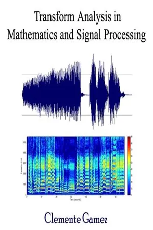
The Discrete Fourier Transform (DFT) is a mathematical technique used to analyze the frequency components of a discrete signal. It converts a sequence of complex numbers representing a time-domain signal into another sequence of complex numbers representing the signal's frequency-domain representation. The DFT is widely used in signal processing, image processing, and various engineering applications for analyzing and manipulating digital data.
Written by Perlego with AI-assistance
Related key terms
1 of 5
12 Key excerpts on "Discrete Fourier Transform"
 No longer available |Learn more
- (Author)
- 2014(Publication Date)
- University Publications(Publisher)
____________________ WORLD TECHNOLOGIES ____________________ Chapter- 4 Discrete Fourier Transform In mathematics, the Discrete Fourier Transform (DFT) is a specific kind of discrete transform, used in Fourier analysis. It transforms one function into another, which is called the frequency domain representation, or simply the DFT , of the original function (which is often a function in the time domain). But the DFT requires an input function that is discrete and whose non-zero values have a limited ( finite ) duration. Such inputs are often created by sampling a continuous function, like a person's voice. Unlike the discrete-time Fourier transform (DTFT), it only evaluates enough frequency components to reconstruct the finite segment that was analyzed. Using the DFT implies that the finite segment that is analyzed is one period of an infinitely extended periodic signal; if this is not actually true, a window function has to be used to reduce the artifacts in the spectrum. For the same reason, the inverse DFT cannot reproduce the entire time domain, unless the input happens to be periodic (forever). Therefore it is often said that the DFT is a transform for Fourier analysis of finite-domain discrete-time functions. The sinusoidal basis functions of the decomposition have the same properties. The input to the DFT is a finite sequence of real or complex numbers (with more abstract generalizations discussed below), making the DFT ideal for processing information stored in computers. In particular, the DFT is widely employed in signal processing and related fields to analyze the frequencies contained in a sampled signal, to solve partial differential equations, and to perform other operations such as convolutions or multiplying large integers. A key enabling factor for these applications is the fact that the DFT can be computed efficiently in practice using a fast Fourier transform (FFT) algorithm. eBook - PDF
- Kamisetty Ramam Rao, Patrick C. Yip, Kamisetty Ramam Rao, Patrick C. Yip(Authors)
- 2018(Publication Date)
- CRC Press(Publisher)
Chapter 2 The Discrete Fourier Transform Ivan W. Selesnick Polytechnic University Gerald Schuller Bell Labs 2.1 Introduction The Discrete Fourier Transform (DFT) is a fundamental transform in digital signal processing, with applications in frequency analysis, fast convolution, image process-ing, etc. Moreover, fast algorithms exist that make it possible to compute the DFT very efficiently. The algorithms for the efficient computation of the DFT are collectively called fast Fourier transforms (FFTs). The historic paper by Cooley and Tukey [15] made well known an FFT of complexity N log 2 N , where N is the length of the data vector. A sequence of early papers [3, 11, 13, 14, 15] still serves as a good reference for the DFT and FFT. In addition to texts on digital signal processing, a number of books devote special attention to the DFT and FFT [4, 7, 10, 20, 28, 33, 36, 39, 48]. The importance of Fourier analysis in general is put forth very well by Leon Co-hen [12]: . . . Bunsen and Kirchhoff, observed (around 1865) that light spectra can be used for recognition, detection, and classification of substances because they are unique to each substance. This idea, along with its extension to other waveforms and the invention of the tools needed to carry out spectral decomposition, certainly ranks as one of the most important discoveries in the history of mankind. The k th DFT coefficient of a length N sequence { x(n) } is defined as X(k) = N − 1 n = 0 x(n) W kn N , k = 0 , . . . , N − 1 (2.1) 37 38 THE Discrete Fourier Transform where W N = e − j 2 π/N = cos 2 π N − j sin 2 π N is the principal N -th root of unity. Because W nk N as a function of k has a period of N , the DFT coefficients { X(k) } are periodic with period N when k is taken outside the range k = 0 , . . . , N − 1. The original sequence { x(n) } can be retrieved by the inverse Discrete Fourier Transform (IDFT) x(n) = 1 N N − 1 k = 0 X(k) W − kn N , n = 0 , . eBook - PDF
Digital Signal Processing
Theory and Practice
- Maurice Bellanger, Benjamin A. Engel(Authors)
- 2024(Publication Date)
- Wiley(Publisher)
35 2 The Discrete Fourier Transform The Discrete Fourier Transform (DFT) is introduced when the Fourier transform of a function is to be calculated using a digital computer. This type of processor can handle only numbers and, in a quantity limited by the size of its memory. It follows that the Fourier transform: S(f ) = ∫ ∞ −∞ s(t)e −j2ft dt must be adapted, by replacing the signal s(t) with the numbers s(nT) which represent a sample of the signal, and by limiting to a finite value N the set of numbers on which the calculations are carried out. The calculation then provides numbers S*(f ) defined by S ∗ (f ) = N−1 ∑ n=0 s(nT)e −j2fnT As the computer has limited processing power, it can only provide results for a limited number of values of the frequency f , and it is natural to choose multiples of a certain frequency step Δf . Thus, S ∗ (kΔf ) = N−1 ∑ n=0 s(nT)e −j2nkΔfT The conditions under which the calculated values form a good approximation to the required values are examined below. An interesting simplifying choice is to take Δf = 1/NT. Then there are only N different values of S*(k/NT), which is a periodic set of period N since: S ∗ [(k + N)∕NT] = S ∗ (k∕NT) On the other hand, the transform thus calculated appears as discrete values and, as shown in Section 1.6, this property is characteristic of the spectrum of periodic functions. Thus, the set S*(k/NT) is obtained by the Fourier transform of the set s(nT), which is periodic, with period NT. The DFT and the inverse transform establish the relations between these two periodic sets. The definition, properties, methods of calculation, and applications of the DFT have been discussed in numerous publications. Overviews are given in References [1–4]. Digital Signal Processing: Theory and Practice, Tenth Edition. Maurice Bellanger. © 2024 John Wiley & Sons Ltd. Published 2024 by John Wiley & Sons Ltd. eBook - PDF
- John H. Karl(Author)
- 2012(Publication Date)
- Academic Press(Publisher)
Application of the Fourier Transform to Digital Signal Processing We have invested in the previous chapter on continuous signal theory because many of the signals that find their way into digital signal processing are thought to arise from some underlying continuous function. In this chapter, we discuss the relationship between these underlying continuous functions and the discrete signals that are produced by their sampling. Fundamental problems will be encountered. A parallel development of the sampling process, in both the time and frequency domains, will clarify these problems and show how to cope with them. However, the deeper insight provided by this development will permit us to evaluate the severity of the limitations encountered in a given circumstance. Finally, after we understand the relationship between the Fourier integral transform and the DFT, new useful ideas will emerge on interpolation, decimation, and modulation. In the preceding chapters, we have pursued a natural course through three kinds of time-frequency transformations. First, evaluation of the frequency response of discrete LSI systems led to the discrete-time/ continuous-frequency description of digital impulse responses and their spectra. Then, by computing this spectra at discrete points in frequency, we were led to the discrete-time/discrete-frequency domain of the DFT. In the last chapter, suitable limits took the DFT over into the Fourier integral transform of continuous time and frequency. To complete our journey into time-frequency transformations, we next address the fourth possibility: continuous time and discrete frequency. 127 7 128 7/ Application of the Fourier Transform Continuous Time, Discrete Frequency: The Fourier Series Discrete spectra are familiar from areas such as spectroscopy, where they are called line spectra. eBook - PDF
- Stan Birchfield(Author)
- 2017(Publication Date)
- Cengage Learning EMEA(Publisher)
All Rights Reserved. May not be copied, scanned, or duplicated, in whole or in part. WCN 02-300 6.2 Discrete Fourier Transform (DFT) 277 (DT F T), on the other hand, applies to signals defined only for discrete values of the domain (but still extending forever), in which case the frequencies are defined only up to the value of 1 2 due to the Nyquist-Shannon sampling theorem just mentioned. In the Fourier series, the roles are reversed, so that the continuous signal is represented as an infinite sum of weighted sinu-soids. Finally, the Discrete Fourier Transform (DF T) applies to signals that have been sampled a finite number of times, so that both the samples and the frequencies are discrete and finite. 6.2 Discrete Fourier Transform (DFT) In this chapter we focus our attention primarily on the last of the four versions, namely, the Discrete Fourier Transform (DFT) . The DF T is arguably the most practical of the versions, since to be stored in a digital computer a continuous signal must be sampled a finite number of times. As a result, all real-world signals are stored as discrete, finite-duration signals, so that if you ever run across the Fourier transform of a real-world signal, you are probably looking at a DF T. Moreover, the discrete mathematics behind the DF T is much simpler than that of the continuous Fourier transform, making it much easier to establish results and recognize connections between different aspects of the theory. One of the nice properties of the DF T is that, unlike some of the other versions, it always exists. † 6.2.1 Forward Transform Let g ( x ) be a 1D discrete signal with w samples. The DF T of g is defined as the summation of the signal after multiplying by a certain complex exponential: G 1 k 2 5 F 5 g 1 x 2 6 5 a w 2 1 x 5 0 g 1 x 2 e 2 j 2 p k x / w (6.13) where x and k are integers. eBook - PDF
Digital Signal Processing
Principles and Applications
- Thomas Holton(Author)
- 2021(Publication Date)
- Cambridge University Press(Publisher)
10 Discrete Fourier Transform (DFT) Introduction In Chapter 3, we showed that there was a unique, invertible relation between a sequence x[n] and its DTFT X(ω): Forward DTFT : X (ω) = F x[n] f g ▵ = X ∞ n = ∞ x[n]e j ωn Inverse DTFT : x[n] = F 1 X (ω) f g ▵ = 1 2π ð 2π ω = 0 X (ω)e j ωn d ω: (10.1) The DTFT is an essential tool for analyzing, understanding and visualizing the response of discrete-time systems. However, because the DTFT is a continuous function of frequency ω, its computation cannot be performed exactly on a digital computer. This limits the utility of the DTFT in many real-world signal-processing operations. As one important example, we showed that convolution of an input signal x[n] and impulse response h[n] could be implemented by multiplication of transforms in the frequency domain, as schematized here: x[n] h[n] = y[n] F# F# F 1 " X (ω) H(ω) = Y (ω) : Specifically, we take the DTFT of x[n] and h[n], multiply the transforms together to form Y(ω), and then take the inverse DTFT to get y[n]. Each of these steps requires operations on the continuous variable ω. In this chapter, we are going to address this limitation of the DTFT. Specifically, we shall show that if we restrict our consideration to a finite-length sequence of length N, x[n], 0 n N 1, then we can completely reconstruct x[n] from only N values of the DTFT. The tool that makes this possible is the Discrete Fourier Transform (DFT). The DFT of x[n], which we denote with the eBook - PDF
- Emiliano R. Martins(Author)
- 2023(Publication Date)
- Wiley(Publisher)
8 The Discrete Fourier Transform (DFT) Learning Objectives In Chapter 7, we found a ‘frequency’ domain representation of discrete signals through the DTFT. The DTFT, however, is itself a continuous function, and as such cannot be implemented in a computer. Thus, to be able to perform operations in the frequency domain using a computer, we need to discretize the DTFT. This discretization leads to the Discrete Fourier Transform (DFT). In Chapter 7, we learned that the consequence of discretizing the time domain is that the frequency domain becomes periodic. In this chapter, we will learn that the consequence of discretizing the frequency domain is that the time domain becomes periodic. This is the key difference between the DFT and the DTFT, and it is crucial to keep it in mind when implementing the former. In this chapter, we will learn how this feature of periodicity in both domains affects the implementation of the DFT and how it connects to the Fourier transform. Importantly, we will learn how to use the function fft, which is a fast implementation of the DFT. With the content covered in this chapter, we will be able to perform operations in both time and frequency domains using a computer. 8.1 Discretizing the Frequency Domain We have seen that a theory of discrete signals and systems is necessary to enable computational analysis. This necessity motivated the definition of a Fourier trans- form of discrete signals, which led to the DTFT. This transformation, however, goes only half-way, because the DTFT is itself a continuous function (v is a contin- uous variable). Consequently, we cannot use a computer to get the inverse DTFT, because the inverse DTFT is an integral, and not a sum. Thus, to be able to perform Essentials of Signals and Systems, First Edition. Emiliano R. Martins. c 2023 John Wiley & Sons Ltd. Published 2023 by John Wiley & Sons Ltd. Companion website: www.wiley.com/go/martins/essentialsofsignalsandsystems
- Robert B. Northrop(Author)
- 2016(Publication Date)
- CRC Press(Publisher)
6 -1 6 The Discrete Fourier Transform 6.1 Introduction The Discrete Fourier Transform (DFT) is the basis for modern spectral analysis of station-ary signals and noise, is used for linear discrete signal processing and filtering, and also one means used to realize joint time-frequency plots used to characterize nonstationary signals (see Chapter 7). In this chapter, we examine the relation of the DFT and inverse DFT (IDFT) to the continuous Fourier transform (CFT), and inverse CFT (ICFT), and describe the mathematical properties of the DFT and IDFT. Also considered are window functions and their role in minimizing the interaction between the spectral components of a sampled signal containing two or more periodic components at different frequen-cies; the choice of window function is shown to affect spectral resolution when calculat-ing the power density spectrogram of a signal. Finally, we introduce the fast Fourier transform (FFT) and illustrate several ways of implementing it. The DFT is used to estimate the spectral (frequency) components of sampled, deter-ministic signals of finite duration, as well as signals and random noise sampled over a finite epoch. When working with sampled, random signals and noise, the DFT can be used to estimate the autopower density spectrum from the autocorrelogram of the finite-duration, sampled waveform. The DFT is also used to calculate the cross-power spectrogram from the cross-correlogram computed from two, finite duration, sampled waveforms: one typically being the input to a linear, time-invariant (LTI) system and the other being the system’s output. The cross-power spectrogram will be shown as useful in estimating the LTI system’s weighting function, or alternately, its frequency response. In Section 6.4, we describe FFT algorithms that offer computational efficiency in cal-culating DFTs, including auto- and cross power spectrograms. eBook - PDF
Signals and Systems
A Primer with MATLAB
- Matthew N. O. Sadiku, Warsame Hassan Ali(Authors)
- 2015(Publication Date)
- CRC Press(Publisher)
272 Signals and Systems: A Primer with MATLAB® recent years has led to digital data communication networks such as local area net-works, metropolitan area networks, and broadband integrated services digital net-works For example, the Internet (the “information superhighway”) allows educators, business people, and others to send electronic mail from their computers worldwide, log onto remote databases, and transfer files A communication engineer designs systems that provide high-quality information services The systems include hardware for generating, transmitting, and receiving information signals More and more government agencies, academic departments, and businesses are demanding faster and more accurate transmission of information To meet these needs, communication engineers are in high demand 6.1 INTRODUCTION In the previous chapters, we have discussed applying frequency-domain techniques to continuous-time signals and systems In this and the next chapter, we consider frequency-domain analysis of discrete-time systems Here, we specifically consider the Fourier analysis of discrete-time systems Fourier analysis plays the same impor-tant role in discrete-time systems as in continuous-time systems Our approach is similar to that used for continuous-time signals and systems We first introduce the discrete-time Fourier transform (DTFT) and its properties We then discuss Discrete Fourier Transform (DFT), and the fast Fourier transform (FFT), a fast method of computing the DFT The DFT plays a vital role in signal processing for spectral, while FFT is the most commonly used Fourier analysis technique The main advantage of DFT and FFT is that they are well suited for computation by a digital computer We learn how to use MATLAB ® to implement numerically the dis-crete Fourier analysis covered in this chapter We finally apply the concepts learned in the chapter to eBook - PDF
- B. P. Lathi, Roger A. Green(Authors)
- 2014(Publication Date)
- Cambridge University Press(Publisher)
This spectrum, shown over more than one period, is depicted in Fig. 9.37 . D [ k ] k Ω 0 9 32 − 2 π − π π 2 π · · · · · · Figure 9.37: Fourier spectrum D [ k ] of a periodic sampled gate function. Example 9.17 By restricting the range of a signal x [ n ] to 0 ≤ n ≤ N − 1, its DFT X [ k ] equals the uniform samples of its DTFT X (Ω). The DTFS, on the other hand, is usually derived assuming that the signal x [ n ] is periodic. As we have seen, however, the DFT and the DTFS are, within a scale factor, mathematically identical to one another. This fact once again reinforces the periodic perspective of the DFT. The DFT is a capable multipurpose tool that handles both the DTFT and the DTFS. Drill 9.18 (DTFS Using an Alternate Frequency Interval) Determine the DTFS of the periodic signal ˜ x [ n ] using the DTFS spectrum of Fig. 9.35 over the interval 2 π < Ω ≤ 4 π . Show that this synthesis is equivalent to that in Eq. (9.58 ). Drill 9.19 (Discrete-Time Fourier Series of a Sum of Two Sinusoids) Find the period N and the DTFS for ˜ x [ n ] = 4 cos(0 . 2 πn ) + 6 sin(0 . 5 πn ). Express the DTFS using D [ k ] computed over 0 ≤ Ω < 2 π . 9.9. Summary 617 Drill 9.20 (Computing the DTFS Spectrum Using the DFT) Using MATLAB and the matrix form of the DFT, compute and plot the DTFS spectrum D [ k ] from Ex. 9.17 . 9.9 Summary The Discrete Fourier Transform (DFT) may be viewed as an economy-class DTFT, applicable when x [ n ] is of finite length. The DFT is one of the most important tools for digital signal processing, es-pecially when we implement it using the efficient fast Fourier transform (FFT) algorithm. Computed using the FFT algorithm, the DFT is truly the workhorse of modern digital signal processing. The DFT X [ k ] of an N -point signal x [ n ] starting at n = 0 represents N uniform samples taken over the frequency interval 0 ≤ Ω < 2 π of X (Ω), the DTFT of x [ n ].
- Michael Corinthios(Author)
- 2018(Publication Date)
- CRC Press(Publisher)
Using duality we have Sd 2 N ( t/ 2) F SC ←→ V n = braceleftBigg 1 − | n | N , − N ≤ n ≤ N 0 , otherwise and Sd 2 N ( t/ 2) F ←→ V ( jω ) = 2 π N summationdisplay n = − N (1 −| n | /N ) δ ( ω − n ) . X 1 ( e j Ω ) = e − j Ω N Sd 2 N (Ω / 2) . 7.30 Fast Fourier Transform The FFT is an efficient algorithm that reduces the computations required for the evaluation of the DFT. In what follows, the derivation of the FFT is developed starting with a simple example of the DFT of N = 8 points. The DFT can be written in matrix form. This form is chosen because it makes it easy to visualize the operations in the DFT and its conversion to the FFT. To express the DFT in matrix form we define an input data vector x of dimension N the elements of which are the successive elements of the input sequence x [ n ]. Similarly we define a vector X of which the elements are the coefficients X [ k ] of the DFT. The DFT X [ k ] = N − 1 summationdisplay n =0 x [ n ] e − j 2 πnk/N (7.186) can thus be written in the matrix form as X = F N x where F N is an N × N matrix of which the elements are given by [ F N ] rs = w rs and w = e − j 2 π N . (7.187) 456 Signals, Systems, Transforms and Digital Signal Processing with MATLAB circleR The inverse relation is written x = 1 N F ∗ N X. (7.188) Note that premultiplication of a square matrix A by a diagonal matrix D producing the matrix C = DA may be obtained by multiplying the successive elements of the diagonal matrix D by the successive rows of A . Conversely, postmultiplication of a square matrix A by a diagonal matrix D producing the matrix C = AD may be obtained by multiplying the successive elements of the diagonal matrix D by the successive columns of A . The following example shows the factorization of the matrix F N , which leads to the FFT. Example 7.32 Let N = 8 . The unit circle is divided as shown in Fig.
- Brad G. Osgood(Author)
- 2019(Publication Date)
- American Mathematical Society(Publisher)
So Z = { 0 , ± 1 , ± 2 , . . . } . 430 7. Discrete Fourier Transform To say a discrete signal is defined on Z N is operationally the same as saying that it’s defined on all the integers, Z , and is periodic of period N . The DFT, with the same definition as before, operates on signals that are defined on Z N and produces signals that are defined on Z N . That’s what a mathematician would say. Adopting this point of view would make some parts of the mathematical devel-opment a little smoother (though no different in substance), but I think it’s extra baggage early on. It doesn’t apply to how we motivated the definition originally (sampling), and in general it can make the tie in with physical applications more awkward. 7.7. Notations and Conventions 2 The definition of the DFT that we’ve given is pretty standard, and it’s the one we’ll use. One sometimes finds an alternate definition of the DFT (used especially in the two-dimensional setting in applications imaging) where N is assumed to be even, and the index set for both the inputs f and the outputs F is taken to be [ − ( N/ 2)+1 : N/ 2] = ( − ( N/ 2)+1 , − ( N/ 2)+2 , . . . , − 1 , 0 , 1 , . . . , N/ 2). There really are N points in that list, and the reason for starting the bottom at − ( N/ 2)+1 and going up to N/ 2 will become clear in a bit. The definition of the DFT is then 5 F f = N/ 2 k = − N/ 2+1 f [ k ] ω − k , or in components F [ m ] = N/ 2 k = − N/ 2+1 f [ k ] ω − km . This puts the k = 0 term in the middle. (In 2D it puts the center of the spectrum of the image at the origin.) We would be led to this indexing of the inputs and outputs if in the sampling-based derivation we originally gave of the DFT, we sampled on the time interval from − L/ 2 to L/ 2 and on the frequency interval from − B to B . Then, using the index set [ − ( N/ 2) + 1 : N/ 2], the sample points in the time domain would be of the form t − N/ 2+1 = − L 2 + 1 2 B = − N/ 2 + 1 2 B , t − N/ 2+2 = − N/ 2 + 2 2 B , .
Index pages curate the most relevant extracts from our library of academic textbooks. They’ve been created using an in-house natural language model (NLM), each adding context and meaning to key research topics.