Inverse Laplace Transform

11 Key excerpts on "Inverse Laplace Transform"

• 

  eBook - PDF

  Numerical and Analytical Methods with MATLAB for Electrical Engineers

  • William Bober, Andrew Stevens(Authors)
  • 2016(Publication Date)
  • CRC Press

    (Publisher)

  201 Chapter 7 Laplace Transforms 7.1 Introduction Transform techniques involve applying a mathematical operation to the equations of a problem, solving in the (presumably easier) transform domain, and then taking the inverse transform to obtain an answer in the domain of interest. Laplace trans-forms are frequently used to solve ordinary and partial differential equations. The method reduces an ordinary differential equation to an algebraic equation, which can be manipulated to a form such that the inverse transform is easily obtained. In circuit theory, any circuit containing capacitors or inductors will contain at least one differential relationship, and a large circuit may contain many more. In Chapter 6, we solved circuits directly in the time domain by integrating the dif-ferential equations in MATLAB. We now describe the Laplace transform approach [1,2]; we convert the time-domain equations to the Laplace domain, solve algebra-ically, and then take the inverse transform back to the time domain to obtain the final answer. Sometimes, we do not even bother with the final step because the result in the Laplace domain is sufficient to fully solve the problem of interest. 7.2 Laplace Transform and Inverse Transform Let f ( t ) be a causal function such that it has some defined value for all t ≥ 0 and is zero otherwise, that is, f ( t ) = 0 for t < 0. The unilateral Laplace transform is defined as L ∫ = = -∞ ( ( )) ( ) ( ) 0 f t F s e f t dt st (7.1) 202 ◾ Numerical and Analytical Methods with MATLAB F ( s ) is called the Laplace transform of f ( t ), and the symbol L is used to indi-cate the transform operation. By convention, we use lowercase letters for time domain functions and uppercase for their Laplace domain (or “ s -domain”) counterparts.

  Sign up to read

  Learn more about book
• 

  eBook - PDF

  Dynamic Systems

  Modeling, Simulation, and Control

  • Craig A. Kluever(Author)
  • 2019(Publication Date)
  • Wiley

    (Publisher)

  Any existing initial conditions of the dynamic system are handled in a systematic manner using the Laplace transformation, and the system’s time response is finally obtained by determining the Inverse Laplace Transform. The reader should recall that we obtained the analytical solution of an LTI differential equation in Chapter 7 by assuming a solution form in the time domain. While this approach is typically the first technique presented in a standard course in differential equations, Laplace transformations offer an alternate approach to solving LTI differential equations “by hand.” 8.2 LAPLACE TRANSFORMATION The Laplace transform converts the function f (t) from the time domain to the domain of the complex variable s, and is defined by ℒ{f (t)} = F(s) = ∫ ∞ 0 f (t)e −st dt (8.1) The Laplace transform variable s =  + j is a complex variable where  and  are the real and imaginary parts, respec- tively. The operation defined by Eq. (8.1) can be stated as “the Laplace transform of f (t) is the complex function F(s).” Typically, the uppercase letter is used for the Laplace transform of the corresponding time function (lowercase letter) and the parenthetical s indicates that the complex (Laplace) variable is the independent variable. The Laplace transform converts an ordinary differential equation (ODE) into an algebraic equation in s, which can be easily manipulated. The inverse operation ℒ −1 {F(s)} = f (t) (8.2) converts the complex function F(s) into the time function f (t) and is known as the “Inverse Laplace Transform of F(s).” Laplace Transforms of Common Time Functions We can use Eq. (8.1) to compute the Laplace transforms of common time functions (such as exponential and sinusoidal functions) and construct a table of these “standard” Laplace transforms. Evaluating the Laplace transformation integral 170 Chapter 8 System Analysis Using Laplace Transforms (Eq. 8.1) requires the mathematical knowledge of an introductory calculus course.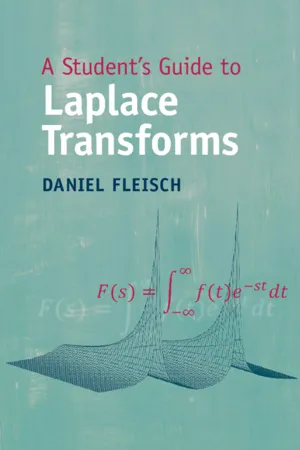

  Sign up to read

  Learn more about book
• 

  eBook - PDF

  A Student's Guide to Laplace Transforms

  • Daniel Fleisch(Author)
  • 2022(Publication Date)
  • Cambridge University Press

    (Publisher)

  1 The Fourier and Laplace Transforms The Laplace transform is a mathematical operation that converts a function from one domain to another. And why would you want to do that? As you’ll see in this chapter, changing domains can be immensely helpful in extracting information from the mathematical functions and equations that describe the behavior of natural phenomena as well as mechanical and electrical systems. Specifically, when the Laplace transform operates on a function f (t) that depends on the parameter t , the result of the operation is a function F(s) that depends on the parameter s . You’ll learn the meaning of those parameters as well as the details of the mathematical operation that is defined as the Laplace transform in this chapter, and you’ll see why the Fourier transform can be considered to be a special case of the Laplace transform. The first section of this chapter (Section 1.1) shows you the mathematical definition of the Laplace transform followed by explanations of phasors, spectra, and the Fourier Transform in Section 1.2. You can see how these trans- forms work in Section 1.3, and you can view transforms from the perspective of linear algebra and inner products in Section 1.4. The relationship between the Laplace frequency-domain function F(s) and the Fourier frequency spectrum F (ω) is presented in Section 1.5, and inverse transforms are described in Section 1.6. As in every chapter, the final section (Section 1.7) contains a set of problems that you can use to check your understanding of the concepts and mathematical techniques presented in this chapter. Full, interactive solutions to every problem are freely available on the book’s website. 1.1 Definition of the Laplace Transform This section is designed to help you understand the answers to the questions “What is the Laplace transform?,” and “What does it mean?” As stated above, 1

  Sign up to read

  Learn more about book
• 

  eBook - PDF

  Numerical and Analytical Methods with MATLAB

  • William Bober, Chi-Tay Tsai, Oren Masory(Authors)
  • 2009(Publication Date)
  • CRC Press

    (Publisher)

  249 12 Chapter Laplace Transforms 12.1 Laplace Transform and Inverse Transform Laplace Transforms [1,2] can be used to solve ordinary and partial differential equa-tions (PDEs). The method reduces an ordinary differential equation to an algebraic equation that can be manipulated to a form such that the inverse transform can be obtained from tables. The inverse transform is the solution to the differential equation. The inverse transform can also be obtained by residue theory in complex variables. The method is applicable to problems where the independent variable domain is from (0 to ∞ ). The method is particularly useful for linear, nonhomoge-neous differential equations, such as vibration problems where the forcing function is piecewise continuous. Let f ( t ) be a function defined for all t ≥ 0 ; then L ( f ( t )) = = -∞ ∫ F s e f t dt s t ( ) ( ) 0 (12.1) F ( s ) is called the Laplace Transform of f ( t ). The inverse transform of F ( s ) is defined to be the function f ( t ) , that is, L -1 ( F ( s )) = f ( t ) (12.2) We can create a table that contains both f ( t ) and the corresponding F ( s ). 250 ◾ Numerical and Analytical Methods with MATLAB Example 12.1 Let f ( t ) = 1; t ≥ 0 . Then L (1) = e dt s t -∞ ∫ 0 = – e s s s t -∞       = 0 1 (12.3) Example 12.2 Let f ( t ) = e at .

  Sign up to read

  Learn more about book
• 

  eBook - PDF

  Linear Circuit Theory

  Matrices in Computer Applications

  • Jiri Vlach(Author)
  • 2016(Publication Date)
  • Apple Academic Press

    (Publisher)

  1 220 Laplace Transformation 9 INTRODUCTION Laplace transformation is the most efficient method for solving linear networks. It was inv ented by Pierre Simon de Laplace in the eighteenth century, but was widely accepted only in the twentieth century. The purpose of a mathematical transformation is to introduce definitions which considerably simplify some complicated steps. In the case of the Laplace transform, dif-ferentiation is replaced by multiplication by the transform variable s . Integration is made even simpler, because it is replaced by division by s . We will not give a fully comprehensive treatment of the Laplace transform theory and only those subjects which have direct relationship to linear networks will be selected. A detailed study is left to specialized mathematical courses. 9.1. DEFINITION OF THE LAPLACE TRANSFORMATION The Laplace transform works with the complex variable s = σ + j ω The real part, σ , does not have any direct practical explanation but the imaginary part does. If we set σ = 0 and thus s = j ω = j 2 π f then we can speak about actual frequency, f, of a steady sinusoidal signal applied to the network. This was already explained in detail in previous Chapters. Let us have a function f ( t ) of time t such that f ( t ) = 0 for t < 0. Then the (one-sided) Laplace transform is defined by L f t F s f t e dt st [ ( )] ( ) ( ) = = -∞ -∫ 0 It is common practice to use capital letters for the transformed variables (functions of s ) and lower case letters for the functions of time, t . (9.1.1) (9.1.2) (9.1.3) Laplace Transformation 221 9.3 9.4 9.5 9.6 9.2 9.1 The inverse transformation is defined by the integral L f t j F s e d s st c j c j -+ -∞ + ∞ = ∫ 1 1 2 [ ( )] ( ) π Note that the inverse transformation has the exponent with + sign and the original trans-formation has – sign. Also note the symbolic notation with L and L –1 . The integration in (9.1.4) is along a line parallel with the imaginary axis.

  Sign up to read

  Learn more about book
• 

  eBook - ePub

  Advanced Mathematical Techniques in Engineering Sciences

  • Mangey Ram, J. Paulo Davim, Mangey Ram, J. Paulo Davim(Authors)
  • 2018(Publication Date)
  • CRC Press

    (Publisher)

  n ), irrational numbers are expressed as a number in fractional power. For a correct understanding of these symbols, examples are given:

  a / b c =

  a

  b c

  ,     a + b / c = a +

  b c

  ,     a /

  (

  b + c

  )

  =

  a

  b + c

  ,     a

  (

  b c + d

  )

  − 1

  =

  a

  b c + d

  ,    

  a

  1 / 2

  = a ,    

  b

  − 1 / 3

  =

  1

  b 3

  .

  1.2   Laplace transform and operations mapping

  The Laplace transform is a powerful mathematical method for solving differential, difference, and integral equations. By means of these equations, one can describe any physical (technological) process and conduct mathematical modeling of the behavior of the object and of the reaction of the environment under the influence of force or other factors, investigate the dynamic properties of the element of construction, and much more.

  In many engineering problems, it is important to investigate a function f (t ), where real variable t is time. Such problems in mechanics relate to dynamic problems.

  The simplest and most economical solution of such problems is possible with the help of methods of the theory of operational calculus [1 ].

  An important role in applied mathematical analysis is played by the Laplace integral

  I =

  ∫ 0 ∞

  f

  ( t )

  e

  − s t

  d t

  .

            (1.1)

  Here, s is a complex variable; s = x + jy ; t > 0.

  To calculate the Laplace integral, the definition and behavior of the function f (t ) for a negative value of the argument t < 0 are immaterial. Therefore, we consider a subclass of piecewise continuous functions f (t ) of the real variable t defined for t > 0 and assumed to be zero for t < 0 (Figure 1.1 ).

  This class of functions is characterized by a certain order of growth, such that for any t > 0 the module f (t ) grows more slowly than some exponential function [1 ].

  Expression (1.1 ) in the operational calculus and its applications is applied in the following form:

  F ( s ) =

  ∫ 0 ∞

  f ( t )

  e

  − s t

  d t

            (1.2)

  Here, the function F (s ) is a function of the complex variable s = x + jy .

  In the new expression (1.2 ), the function of the complex variable s is put in correspondence with the function of the real variable t

  Sign up to read

  Learn more about book
• 

  eBook - PDF

  Essentials of Advanced Circuit Analysis

  A Systems Approach

  • Djafar K. Mynbaev(Author)
  • 2024(Publication Date)
  • Wiley

    (Publisher)

  We solve this equation for V( ) s , as shown in Box 4. To convert V s ( ) back into the time-domain formulas, we apply the Inverse Laplace Transform, L −1 { ( )} ( ), V s v t = and use Table 7.1. Thus, L s e t − − +               = 1 2 12 2 12 ( ) and L s e t − − − +               =− 1 3 10 3 10 ( ) . Their sum gives us the required solution of the given differential equa- tion in the time domain, v t e e t t ( ) = − − − 12 10 2 3 , as shown in Box 2. Now, we can see that obtaining the system’s response by employing the Laplace transform is much easier than resorting to the integration of the system’s differential equation. (Note that Figure 7.3 shows v t in ( ) = 0 . In fact, v t in ( ) could be any; we’ve chosen the simplest case to not overshadowing the main concept of the Laplace transform by extraneous mathematical manipulations.) Unhappily, no benefit comes for free: The price for gaining this advantage is the need for addi- tional operations: direct and Inverse Laplace Transforms. Nevertheless, overall, the use of the Laplace transform is well worth undertaking these additional operations. In short, remember this: The Laplace transform method is a powerful tool for obtaining a circuit’s response—a task we carried out throughout this textbook. 7.2.4 Examples of the Laplace Transform Operations Let’s consider the examples of Laplace transform operations. Applying the Laplace transform to time-domain functions to obtain their s-domain equivalents is a straightforward operation: We just need to use the rules in Tables 7.1. To demonstrate this operation, several examples are assembled Figure 7.3 The concept of the Laplace transform method. 7 What and Why of the Laplace Transform 380 in Table 7.2. In this table, at the Laplace transform side, we first show the general rule of the Laplace transform to be used and then demonstrate this rule’s application to a specific example.

  Sign up to read

  Learn more about book
• 

  eBook - PDF

  Engineering Circuit Analysis

  • J. David Irwin, R. Mark Nelms(Authors)
  • 2022(Publication Date)
  • Wiley

    (Publisher)

  C H A P T E R 12 12 12.1 ❯ Definition The Laplace transform of a function f (t) is defined by the equation ℒ[ f (t)] = F(s) =  0 ∞ f (t)e −st dt (12.1) where s is the complex frequency s = σ + jω (12.2) and the function f (t) is assumed to possess the property that f (t) = 0 for t < 0 Note that the Laplace transform is unilateral (0 ≤ t < ∞), in contrast to the Fourier transform (see Chapter 14), which is bilateral (−∞ < t < ∞). In our analysis of circuits using the Laplace transform, we will focus our attention on the time interval t ≥ 0. It is the initial conditions that account for the operation of the circuit prior to t = 0; therefore, our analyses will describe the circuit operation for t ≥ 0. For a function f (t) to possess a Laplace transform, it must satisfy the condition  0 ∞ e −σt | f (t) | dt < ∞ (12.3) for some real value of σ. Because of the convergence factor e −σt , a number of important func- tions have Laplace transforms, even though Fourier transforms for these functions do not exist. All of the inputs we will apply to circuits possess Laplace transforms. Functions that do not have Laplace transforms ( e.g., e t 2 ) are of no interest to us in circuit analysis. The Inverse Laplace Transform, which is analogous to the inverse Fourier transform, is defined by the relationship ℒ −1 [F(s)] = f (t) = 1 ___ 2πj  σ 1 −j∞ σ 1 +j∞ F (s)e st ds (12.4) where σ 1 is real and σ 1 > σ in Eq. (12.3). The Laplace Transform LEARNING OBJECTIVES The learning goals for this chapter are that students should be able to: ❯ Determine the Laplace transform of signals commonly found in electric circuits. ❯ Perform the Inverse Laplace Transform using partial fraction expansion. ❯ Describe the concept of convolution. ❯ Apply the initial-value and final-value theorems to determine the voltages and currents in an ac circuit. ❯ Use the Laplace transform to analyze transient circuits.

  Sign up to read

  Learn more about book
• 

  eBook - PDF

  A Course in Ordinary Differential Equations

  • Stephen A. Wirkus, Randall J. Swift(Authors)
  • 2014(Publication Date)
  • Chapman and Hall/CRC

    (Publisher)

  (7.41) These remarks allow another method for computing inverse Laplace trans-forms. Suppose we are given a function H and need to find L -1 { H ( s ) } . If we can express H ( s ) as a product F ( s ) G ( s ) where L -1 { F ( s ) } = f ( t ) and L -1 { G ( s ) } = g ( t ) are known, then we can apply (7.40) or (7.41) to determine L -1 { H ( s ) } . Example 2: Find L -1 n 1 s ( s 2 +1) o using the convolution and the transform table. 7.7. The Convolution 561 Solution Writing 1 s ( s 2 +1) as the product F ( s ) G ( s ) where F ( s ) = 1 s and G ( s ) = 1 s 2 + 1 we have by Table 7.1 f ( t ) = L -1 1 s = 1 and g ( t ) = L -1 1 s 2 + 1 = sin t so L -1 1 s ( s 2 + 1) = f ( t ) * g ( t ) = Z t 0 1 · sin( t -τ ) dτ or L -1 1 s ( s 2 + 1) = g ( t ) * f ( t ) = Z t 0 sin τ · 1 dτ. Here the second integral is (slightly) more simple to evaluate, so we have L -1 1 s ( s 2 + 1) = 1 -cos t. Note that we obtained this result earlier by means of a partial fractions de-composition. Example 3: Newton’s Law of Cooling (revisited) Solution Recall from Chapter 1 we considered Newton’s Law of Cooling: dT dt = k [ T ( t ) -T s ( t )] , which says that the rate of change of the temperature T ( t ) of a body is proportional to the difference between the temperature of the body and its surroundings T s ( t ). Unlike our work in Chapter 1, here we assume T s is not necessarily a constant. So, applying the Laplace transform to both sides of this differential equation gives L dT dt = L{ k [ T ( t ) -T s ( t )] } which is s L{ T } -T (0 -) = k L{ T } -k L{ T s } . 562 Chapter 7. Laplace Transforms Solving this equation for L{ T } gives L{ T } = T (0 -) s -k -k s -k L{ T s } . Using the convolution theorem we find the Inverse Laplace Transform as T ( t ) = T (0 -) e kt -Z t 0 -kT s ( z ) e k ( t -z ) dz, that is, T ( t ) = T (0 -) e kt -ke kt Z t 0 -T s ( z ) e -kz dz. (7.42) Equation (7.42) is the solution of Newton’s Law of Cooling with a nonconstant surrounding temperature.

  Sign up to read

  Learn more about book
• 

  eBook - PDF

  A Course in Differential Equations with Boundary Value Problems

  • Stephen A. Wirkus, Randall J. Swift, Ryan Szypowski(Authors)
  • 2017(Publication Date)
  • CRC Press

    (Publisher)

  (7.41) These remarks allow another method for computing Inverse Laplace Transforms. Suppose we are given a function H and need to find L -1 {H(s)}. If we can express H(s) as a product F (s)G(s) where L -1 {F (s)} = f (t) and L -1 {G(s)} = g(t) are known, then we can apply (7.40) or (7.41) to determine L -1 {H(s)}. Example 2 Find L -1  1 s(s 2 +1)  using the convolution and the transform table. Solution Writing 1 s(s 2 +1) as the product F (s)G(s) where F (s) = 1 s and G(s) = 1 s 2 + 1 we have, by Table 7.1, f (t) = L -1  1 s  = 1 and g(t) = L -1  1 s 2 + 1  = sin t so L -1  1 s(s 2 + 1)  = f (t) * g(t) =  t 0 1 · sin(t - τ ) dτ or L -1  1 s(s 2 + 1)  = g(t) * f (t) =  t 0 sin τ · 1 dτ. Here the second integral is (slightly) more simple to evaluate, so we have L -1  1 s(s 2 + 1)  = 1 - cos t. Note that we obtained this result earlier by means of a partial fractions decomposition. 468 Chapter 7. Laplace Transforms Example 3 Newton’s Law of Cooling (revisited) Solution Recall from Chapter 1 we considered Newton’s law of cooling: dT dt = k[T (t) - T s (t)], which says that the rate of change of the temperature T (t) of a body is proportional to the difference between the temperature of the body and its surroundings T s (t). Unlike our work in Chapter 1, here we assume T s is not necessarily a constant. So, applying the Laplace transform to both sides of this differential equation gives L  dT dt  = L{k[T (t) - T s (t)]} which is sL{T }- T (0 - ) = kL{T }- kL{T s }. Solving this equation for L{T } gives L{T } = T (0 - ) s - k - k s - k L{T s }. Using the convolution theorem, we find the Inverse Laplace Transform as T (t) = T (0 - )e kt -  t 0 - kT s (z)e k(t-z) dz, that is, T (t) = T (0 - )e kt - ke kt  t 0 - T s (z)e -kz dz. (7.42) Equation (7.42) is the solution of Newton’s law of cooling with a nonconstant surrounding temperature.

  Sign up to read

  Learn more about book
• 

  eBook - PDF

  Introductory Signal Processing

  • Roland Priemer(Author)
  • 1990(Publication Date)
  • WSPC

    (Publisher)

  LTI SYSTEM ANALYSIS WITH THE LAPLACE TRANSFORM 419 C ^ + ^ p ^ + ^ ^ = 0 (833) dt R 2 R t v L (0-v c (0 1 f< p ■ , f l v L Wx+/ 0 = 0 (8.34) Here we have two coupled differential-integral equations. Taking the Laplace transform results in cCsV ( /Cs)-V 0 )+ + = 0 VL(^)-V C (5) 1 7 0 R 2 Ls s These equations can now be manipulated to solve for V c (s ) in terms of V(s ) and the initial conditions. Let R 1 =R 2 =l,L = l, and C = 1, and after eliminating VJXS), we have ^ 2 +25+2 ,s 2 +2s+2 Now, we can recognize the input-output transfer function, the zero-state response, the zero-input response, and the natural frequencies of the system. And, we can find the complete response v c (t)withv c (t)=L-V c (s)). Or, from V c (s) = H(s)V(s), the overall input-output differential equation is given by d 2 v c (t) dv c {t) dv(t) / x _ + 2 — + 2 ^ ( 0 = -^ + v ( 0 To solve this equation, we need the initial conditions v c (0) and dv c /dt at t = 0. If in eq. 8.34 we set t = 0~, then we have v L (01 = v c (0-)-/? 2 / 0 = y 0 -^ 0 and from eq. 8.33 we get for t = 0 dv r lfv r (0~) ( h V 0 dv c . lfv L ((T) (1 1 } h V 0 Now, we could proceed to solve the second order differential equation for v c (r). Example 8.18. In this example we will skip writing time domain equations, and immediately write frequency domain equations in terms of component impedances and the transforms of the node voltages. The circuit we will consider is shown in Fig. 8.9. 420 INTRODUCTORY SIGNAL PROCESSING The device labeled with a is an ideal amplifier, and v 4 (f) = ccv 3 (f) or V 4 (s) = aV 3 (s). As we will see, the entire circuit behaves as a low-pass filter. However, other circuits involving RC components and amplifiers can be designed to achieve a great variety of filtering characteristics.

  Sign up to read

  Learn more about book