Structural Equation Modeling with Mplus

Basic Concepts, Applications, and Programming

Barbara M. Byrne

• Editore: Routledge
• Anno: 2013
• ISBN:
  9781136663451
• Edizione: 1
• Argomento: Psychology
• Categoria: Research & Methodology in Psychology

Modeled after Barbara Byrne's other best-selling structural equation modeling (SEM) books, this practical guide reviews the basic concepts and applications of SEM using M plus Versions 5 & 6. The author reviews SEM applications based on actual data taken from her own research. Using non-mathematical language, it is written for the novice SEM user. With each application chapter, the author "walks" the reader through all steps involved in testing the SEM model including:

• an explanation of the issues addressed
• illustrated and annotated testing of the hypothesized and post hoc models
• explanation and interpretation of all M plus input and output files
• important caveats pertinent to the SEM application under study
• a description of the data and reference upon which the model was based
• the corresponding data and syntax files available under "Supplementary Material" below

The first two chapters introduce the fundamental concepts of SEM and important basics of the M plus program. The remaining chapters focus on SEM applications and include a variety of SEM models presented within the context of three sections: Single-group analyses, Multiple-group analyses, and other important topics, the latter of which includes the multitrait-multimethod, latent growth curve, and multilevel models.

Intended for researchers, practitioners, and students who use SEM and M plus, this book is an ideal resource for graduate level courses on SEM taught in psychology, education, business, and other social and health sciences and/or as a supplement for courses on applied statistics, multivariate statistics, intermediate or advanced statistics, and/or research design. Appropriate for those with limited exposure to SEM or M plus, a prerequisite of basic statistics through regression analysis is recommended.

section II

Single-Group Analyses

Confirmatory Factor Analytic Models

Chapter 3. Testing the Factorial Validity of a Theoretical Construct (First-Order CFA Model)

Chapter 4. Testing the Factorial Validity of Scores From a Measuring Instrument (First-Order CFA Model)

Chapter 5. Testing the Factorial Validity of Scores From a Measuring Instrument (Second-Order CFA Model)

The Full Latent Variable Model

Chapter 6. Testing the Validity of a Causal Structure

chapter 3

Testing the Factorial Validity
of a Theoretical Construct

First-Order Confirmatory
Factor Analysis Model

Our first application examines a first-order confirmatory factor analysis (CFA) model designed to test the multidimensionality of a theoretical construct. Specifically, this application tests the hypothesis that self-concept (SC), for early adolescents (grade 7), is a multidimensional construct composed of four factors—General SC (GSC), Academic SC (ASC), English SC (ESC), and Mathematics SC (MSC). The theoretical underpinning of this hypothesis derives from the hierarchical model of SC proposed by Shavelson, Hubner, and Stanton (1976). The example is taken from a study by Byrne and Worth Gavin (1996) in which four hypotheses related to the Shavelson et al. model were tested for three groups of children—preadolescents (grade 3), early adolescents (grade 7), and late adolescents (grade 11). Only tests bearing on the multidimensional structure of SC, as it relates to grade 7 children, are relevant in the present chapter. This study followed from earlier work in which the same four-factor structure of SC was tested for adolescents (see Byrne & Shavelson, 1986) and was part of a larger study that focused on the structure of social SC (Byrne & Shavelson, 1996). For a more extensive discussion of the substantive issues and the related findings, readers should refer to the original Byrne and Worth Gavin article.

The Hypothesized Model

In this first application, the inquiry focuses on the plausibility of a multidimensional SC structure for early adolescents. Although such dimensionality of the construct has been supported by numerous studies for grade 7 children, others have counterargued that SC is less differentiated for children in their pre- and early adolescent years (e.g., Harter, 1990). Thus, the argument could be made for a two-factor structure comprising only GSC and ASC. Still others postulate that SC is a unidimensional structure, with all SC facets embodied within a single SC construct (GSC).

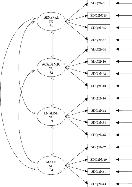
Figure 3.1. Hypothesized four-factor CFA model of self-concept.

(For a review of the literature related to these issues, see Byrne, 1996.) The task presented to us here, then, is to test the original hypothesis that SC is a four-factor structure comprising a general component (GSC), an academic component (ASC), and two subject-specific components (ESC and MSC), against two alternative hypotheses: (a) that SC is a two-factor structure comprising GSC and ASC, and (b) that SC is a one-factor structure in which there is no distinction between general and academic SCs.

We turn now to an examination and testing of each of these hypotheses.

Hypothesis 1: Self-Concept Is a Four-Factor Structure

The model to be tested in Hypothesis 1 postulates a priori that SC is a four-factor structure composed of General SC (GSC), Academic SC (ASC), English SC (ESC), and Math SC (MSC); it is presented schematically in Figure 3.1.

Before any discussion of how we might go about testing this model, let's take a few minutes first to dissect the model and list its component parts as follows:

• There are four SC factors, as indicated by the four ovals labeled General SC, Academic SC, English SC, and Math SC.
• The four factors are correlated, as indicated by the two-headed arrows.
• There are 16 observed variables, as indicated by the 16 rectangles (SDQ2N01 through SDQ2N43); they represent item pairs¹ from the General, Academic, Verbal, and Math SC subscales of the Self-Description Questionnaire II (SDQ2; Marsh, 1992).
• The observed variables load on the factors in the following pattern: SDQ2N01 to SDQ2N37 load on Factor 1, SDQ3N04 to SDQ2N40 load on Factor 2, SDQ2N10 to SDQ2N46 load on Factor 3, and SDQ2N07 to SDQ2N42 load on Factor 4.
• Each observed variable loads on one and only one factor.
• Residuals associated with each observed variable are uncorrelated.

Summarizing these observations, we can now present a more formal description of our hypothesized model. As such, we state that the CFA model presented in Figure 3.1 hypothesizes a priori that

1. SC responses can be explained by four factors: General SC, Academic SC, English SC, and Math SC;
2. each item-pair measure has a nonzero loading on the SC factor that it was designed to measure (termed a target loading) and a zero loading on all other factors (termed nontarget loadings);
3. the four SC factors, consistent with the theory, are correlated; and
4. residual errors associated with each measure are uncorrelated.

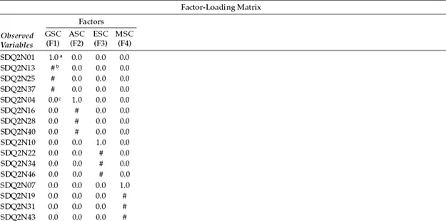
Another way of conceptualizing the hypothesized model in Figure 3.1 is within a matrix framework as presented in Table 3.1. Thinking about the model components in this format can be very helpful because it is consistent with the manner by which the results from structural equation modeling (SEM) analyses are commonly reported in program output files. The tabular representation of our model in Table 3.1 shows the pattern of parameters to be estimated within the framework of three matrices: the factor-loading matrix, the factor variance–covariance matrix, and the residual variance–covariance matrix. In statistical language, these parameter arrays are termed the lambda, psi, and theta matrices, respectively. We will revisit these matrices later in the chapter in discussion of the TECH1 Output option.

Table 3.1 Pattern of Estimated Parameters for Hypothesized Four-Factor Model

a Parameter fixed to 1.0.

b Parameter to be estimated.

c Parameter fixed to 0.0.

For purposes of model identification and latent variable scaling (see Chapter 2), you will note that the first of each congeneric set (see Chapter 2, note 2) of SC measures in the factor-loading matrix is set to 1.0, which you may recall is default in Mplus; all other parameters are freely estimated (as represented by the pound sign: #). Likewise, as indicated in the factor variance–covariance matrix, all parameters are freely estimated. Finally, in the residual variance–covariance matrix, only the residual variances are estimated; all residual covariances are presumed to be zero.

Provided with these two views of this hypothesized four-factor model, let's now move on to the testing of this model. We begin, of course, by structuring an input file that fully describes the model to Mplus.

Mplus Input File Specification and Output File Results

Input File Specification

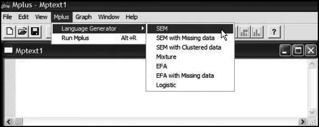
In Chapter 2, I advised you of the Mplus language generator and provided a brief description of its function and limitations, together with an illustration of how this facility can be accessed. In this first application, I now wish to illustrate how to use this valuable feature by walking you through the steps involved in structuring the input file related to Figure 3.1. Following from the language generator menu shown in Figure 2.2, we begin by clicking on the SEM option as illustrated in Figure 3.2.

Figure 3.2. Mplus language generator: Selecting category of analytic model.

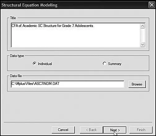
Figure 3.3. Mplus language generator: Specification of title and location of data.

Once you click on the SEM option, you will be presented with the dialog box shown in Figure 3.3. Here I have entered a title for the model to be tested (see Figure 3.1), indicated that the data represent individual scores, and provided the location of the data file on my computer. The Browse button simplifies this task.

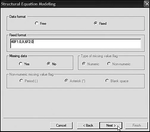
The next dialog box presented to you (see Figure 3.4) requests information related to the data: (a) whether they are in free or fixed format and, if the latter, specifics of the Fortran statement format state; and (b) if there are any missing data. The data to be used in this application (ascindm.dat) are in fixed format as noted, and the format statement is 40F1.0, X, 6F2.0. This expression tells the program to read 40 single-digit numbers, to skip one column, and then to read six double-digit numbers. The first 40 columns represent item scores on the Self-Perception Profile for Children (SPPC; not used in the present study) and the SDQ2; the remaining six scores represent scores for the MASTENG1 through SMAT1 variables (not used in the present study). Finally, we note that there are no missing data.

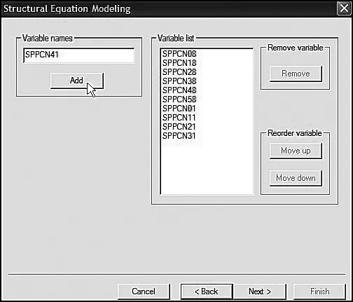
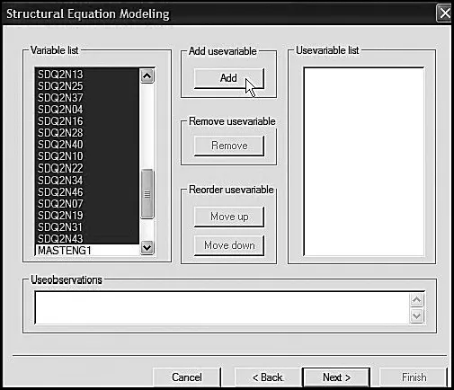
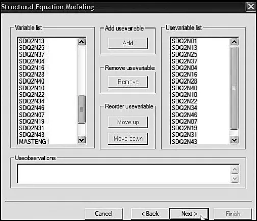
The next three dialog boxes (Figures 3.5, 3.6, and 3.7) focus on the variable names. The first dialog box, shown in Figure 3.5, requests the names of all variables in the entire data set. Here you can see that they are first entered and then added to the list one at a time. In the dialog box shown in Figure 3.6, you are asked to specify which variables will actually be used in the analyses. Shown on the left side of this dialog box, you can see that I have blocked this specific set of variables, which is now ready for transfer over to the Usevariable List. Finally, Figure 3.7 shows the completion of this process.

Figure 3.4. Mplus language generator: Specification of fixed format for data.

Figure 3.5. Mplus language generator: Specification and adding all observed variables in the data to the variable list.

Figure 3.6. Mplus language generator: Selected observed variables to be used in the analyses.

Figure 3.7. Mplus language generator: Addition of selected observed variables to the usevariable list.

The next two dialog boxes, in the present instance, do not require any additional input information; nonetheless, it is important that I show them to you in the interest of your own work in the future. The dialog box shown in Figure 3.8 provides the opportunity of specifying (a) a grouping variable, which is not applicable to the present analyses; (b) a weight variable, which is not applicable; and (c) existing categorical variables; all variables in the present data set are of continuous scale. The dialo...