Tracking with Particle Filter for High-dimensional Observation and State Spaces

Séverine Dubuisson

• Publisher: Wiley-ISTE
• Year: 2015
• Print ISBN: 9781848216037
• eBook ISBN: 9781119054054
• Edition: 1
• Topic: Technology & Engineering
• Subtopic: Signals & Signal Processing
• Index: Technology & Engineering

This title concerns the use of a particle filter framework to track objects defined in high-dimensional state-spaces using high-dimensional observation spaces. Current tracking applications require us to consider complex models for objects (articulated objects, multiple objects, multiple fragments, etc.) as well as multiple kinds of information (multiple cameras, multiple modalities, etc.). This book presents some recent research that considers the main bottleneck of particle filtering frameworks (high dimensional state spaces) for tracking in such difficult conditions.

1

Visual Tracking by Particle Filtering

1.1. Introduction

The aim of this introductory chapter is to give a brief overview of the progress made over the last 20 years in visual tracking by particle filtering. To begin (section 1.2), we will present the theoretical elements necessary for understanding particle filtering. Thus, we will first introduce recursive Bayesian filtering, before giving the outline of particle filtering. For more details, in particular theorem demonstrations and convergence studies, we invite the reader to refer to more advanced studies [CHE 03b, DOU 00b, GOR 93]. We will then explain how particle filtering is used in visual tracking in video sequences. Although the literature is abundant on this subject and evolving very fast, it is impossible to give a complete overview of this subject. Next, section 1.3 presents certain limits of particle filtering. Toward the end, we specify our scientific position in section 1.4 and the methodological axes that allow a part of these problems to be solved. Finally, section 1.5 gives the current state of the main large families of approaches that are concerned with managing large-sized state and/or observation spaces in particle filtering.

1.2. Theoretical models

1.2.1. Recursive Bayesian filtering

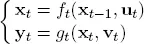
Recursive Bayesian filtering [JAZ 70] aims to approximate the state of a hidden Markov process, which is observed through an observation equation. Let {x_0:t} = {x₀, . . . , x_t} be this process, where x_t is the state vector, y_t the observation at instant t and the two models:

[1.1]

The first equation is the state equation, with the state transition function f_t between the instants t – 1 and t, and the second is the observation equation, giving the measurement of the state through an observation function g_t. u_t and v_t are independent white noises.

All information necessary for approximating x_0:t is contained in the a posteriori density, also known as the filtering density, p(x_0:t|y_1:t), where y_1:t = {y₁,y₂, . . . ,y_t}, in which we can prove, by applying the definition of conditional probabilities, that it follows the following recursive equation for a known [CHE 03b] t ≥ 1 (p(x₀):

[1.2]

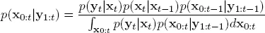
Under the Markov hypothesis, p(y_t|y_1:t–1,x_0:t) = p(y_t|x_t) (the observations at different instants are independent between themselves given the states and do not depend on the state at the current instant) and p(x_t|x_0:t–1, y_1:t–1) = p(x_t|x_t–1) (the current state only depends on the previous state), equation [1.2] becomes:

[1.3]

The state transition equation is represented by the density p(x_t|x_t–1) and is linked to the f_t function. This density is also called the transition function and gives the probably state x_t at the instant t, given its previous state x_t–1. The observation equation is represented by p(y_t|x_t) and is linked to the function g_t. This density is also called the likelihood function and gives the probability of making the observation y_t given the state x_t. We can see that equation [1.3] is recursive and it decomposes into two primary stages that we detail below.

1) The first stage, known as prediction step, allows approximating the a posteriori density p(x_0:t|y_1:t–1) using the transition distribution p(x_t|x_t–1) and the previously approximated density p(x_0:t–1|y_1:t–1).

2) The second stage, called correction step, allows obtaining the a posteriori density p(x_0:t|y_1:t), using the likelihood distribution p(y_t|x_t), which depends on the new observation. This a posteriori density represents the density of the probability to have the set of states x_0:t, among all the possible states, given the history of the observations y_1:t.

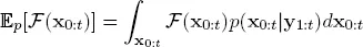
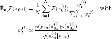
In order to obtain calculable estimators of x_0:t, we can use, for example, the conditional mean, given by:

[1.4]

where

is some bounded function. If the densities are Gaussian, then there exists a solution (analytical expression of the Gaussian parameters to approximate) given by the Kalman filter [KAL 60]. Otherwise, the whole of equation [1.4] is not calculable directly. We can invoke, under special conditions, the solutions given by the following types of methods:

– analytical (extended Kalman filter [JAZ 70], unscented Kalman filter [JUL 97]) that approach the law from a Gaussian sum and are better adapted to weakly nonlinear and unimodal cases, which is nonetheless not appropriate for most problems of vision;

– numerical (approximations by discrete tables, division into parts) that are, most of the time, complex to solve, not very flexible and only adapted to state spaces of a small size.

Most of the time, in vision, solutions are not adapted as the integrals are not directly calculable. For the general case (non-parametric and multi-modal densities), it is necessary to make use of numerical approximations, such as those provided by sequential Monte-Carlo methods, which we will present in the following section and that are the methodological heart of this work.

1.2.2. Sequential Monte-Carlo methods

Sequential Monte-Carlo methods, also known under the name of particle filters (PFs), were studied by many researchers at the beginning of the 1990s [GOR 93, MOR 95] and combine Monte-Carlo simulation and recursive Bayesian filtering. Today, they are widely used in the computer visualization community. Before detailing the principle of particle filtering, we need to introduce importance sampling.

1.2.2.1. Importance sampling

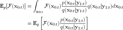
Once the a posteriori density defined by equation [1.3] has been approximated, we can evaluate the estimator given in equation [1.4]. The Monte-Carlo method allows us to approximate this integral with the realization of a random variable distributed according to the a posteriori density. Unfortunately, we are almost never able to sample following this law, so to solve this problem, we introduce a proposal function (or importance function) q(x_0:t|y_1:t), whose support contains p(x_0:t|y_1:t) and from which we can sample. The conditional mean is then given by:

[1.5]

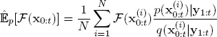
With N realizations

~ q(x_0:t|y_1:t), i = 1, . . . , N, we can approximate the previous estimator by:

[1.6]

The law of large numbers allows us to show that this estimator almost certainly converges toward

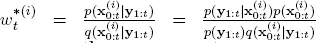
(x_0:t)] when N tends to infinity. Thus, we define the importance weights by

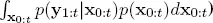
, whose expression requires the calculation of the integral (p(y_1:t) =

p(y_1:t|x_0:t)p(x_0:t)dx_0:t), which is generally impossible. We can nevertheless show that the following equation is usable [DOU 01]:

[1.7]

This estimator almost certainly converges when N tends to infinity. Then, it is sufficient to make the importance sampling recursive, to obtain the particle filtering algorithm described below.

1.2.2.2. Particle filter

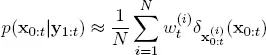
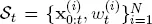
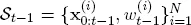
The idea is thus to represent and to approximate empirically the a posteriori density by a weighted sample of size N

, i = 1, … , N such that:

[1.8]

where the individuals

, also called particles, are the realizations of the random variable x_0:t (state of the object) in the state space (δ being the Dirac function). Every particle is therefore a possible solution of the state to approximate and its associated weight represents its quality according to the available observations. Hence, the sample

at the instant t is calculated from the previous sample

, so as to obtain an approximation (via sampling) of the filtering density p(x_0:t|y_1:t) at the current instant. For this, three stages are necessary: i) a state exploration stage, during which we propagate the particles via the proposal function, ii) a stage for the evaluation (or the correction) of the particle quality, which aims to calculate their new weight and finally iii) an optional stage for particle selection (re-sampling). The generic particle filtering scheme (SIR filter – sequential importance resampling), between the instants t – 1 and t, is summarized in th...

Table of contents

• Cover Page
• Contents
• Title Page
• Copyright Page
• Notations
• Introduction
• 1. Visual Tracking by Particle Filtering
• 2. Data Representation Models
• 3. Tracking Models That Focus on the State Space
• 4. Models of Tracking by Decomposition of the State Space
• 5. Research Perspectives in Tracking and Managing Large Spaces
• Bibliography
• Index