VaR Methodology for Non-Gaussian Finance

Marine Habart-Corlosquet, Jacques Janssen, Raimondo Manca

• Publisher: Wiley-ISTE
• Year: 2013
• Print ISBN: 9781848214644
• eBook ISBN: 9781118733981
• Edition: 1
• Topic: Commerce
• Subtopic: Finance

With the impact of the recent financial crises, more attention must be given to new models in finance rejecting "Black-Scholes-Samuelson" assumptions leading to what is called non-Gaussian finance. With the growing importance of Solvency II, Basel II and III regulatory rules for insurance companies and banks, value at risk (VaR) – one of the most popular risk indicator techniques plays a fundamental role in defining appropriate levels of equities. The aim of this book is to show how new VaR techniques can be built more appropriately for a crisis situation.

VaR methodology for non-Gaussian finance looks at the importance of VaR in standard international rules for banks and insurance companies; gives the first non-Gaussian extensions of VaR and applies several basic statistical theories to extend classical results of VaR techniques such as the NP approximation, the Cornish-Fisher approximation, extreme and a Pareto distribution. Several non-Gaussian models using Copula methodology, Lévy processes along with particular attention to models with jumps such as the Merton model are presented; as are the consideration of time homogeneous and non-homogeneous Markov and semi-Markov processes and for each of these models.

1

Use of Value-at-Risk (VaR) Techniques for Solvency II, Basel II and III

In recent years, banks and insurance companies have been subjected to more and more regulations in order to increase transparency of their risk management and to minimize the risk of bankruptcy. On the one hand, Basel II (in 2004) and Basel III in (2010), which are, respectively, the second and third of the Basel Accords, are international recommendations on banking laws and regulations issued by the Basel Committee on Banking Supervision. On the other hand, the Solvency II Directive is a European Directive that codifies and harmonizes the European insurance regulation. Solvency II is currently scheduled to come into effect on January 1, 2014. These two standards aim at measuring the solvability of banks or insurance companies in time intervals (one day, 10 days, one year, etc.). To do so, both standards use the value at risk (VaR) concept. This chapter discusses the importance of the VaR in these international standards and the restrictive assumptions under which this concept is used.

1.1. Basic notions of VaR

1.1.1. Definition

Formally, VaR measures the worst expected loss over a given horizon under normal market conditions at a given confidence level. For example, a daily VaR of $30 million at a 99% confidence level means that there is only one chance in 100, under normal market conditions, for a loss greater than $30 million to occur. Usual time horizons are one day, one month or one year. Usual confidence levels are 95%, 99% or 99.5%.

VaR at level α, with ∞∈]0,1[ , is mathematically defined by the quantile of the random variable X under the probability distribution P, as shown in the following formula:

[1.1]

VaR is based on three key parameters: the probability distribution of losses, the time horizon and the confidence level.

The probability distribution of losses depends on the underlying portfolio (e.g. assets held by a bank or an insurance company, or the claims of a portfolio of insured people). This probability distribution of losses is generally difficult to estimate at best, in particular when the underlying portfolio is heterogeneous (e.g. if the portfolio is composed of many different types of asset).

Choosing a consistent time horizon depends on four major criteria. First, the time horizon chosen must match the holding period of the underlying portfolio to assess. This is the reason there is a major difference between banks and insurance companies. Whereas the time horizon is short term for banks (a few days), it is long term for insurance companies (the duration of the liabilities is often close to eight years). Second, portfolio composition should remain unchanged on the time horizon. This is verified in the context of Solvency II and Basel II–III because the portfolios are valued in runoff. Third, the time horizon chosen should be consistent with the degree of risk aversion of the bank or insurance company. Fourth, the time horizon chosen must be the same across the several institutions that we would like to compare. This implies that supervisors set a time horizon common to all banks or all insurance companies in order to compare them.

The confidence level depends on three major criteria. First, the confidence level obviously depends on the risk aversion of the bank or insurance company. Second, as for the time horizon, the confidence level must be the same across the several institutions that we would like to compare. Third, for reliable risk management, defining a relatively low threshold is better so as to obtain observations of overtaking and to check the robustness of the calculation.

1.1.2. Calculation methods

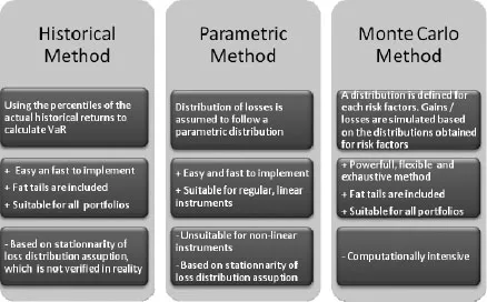
In this section, we not only give a comprehensive analysis of VaR, but also briefly discuss the different methods for its calculation, which are fully discussed in the subsequent chapters both in the fields of Gaussian and non-Gaussian finance. Although VaR is a very intuitive concept, its measurement is a challenging statistical problem. Three methods are available for the calculation of VaR: the historical, the parametric and the Monte Carlo methods. All these three methods have their own strengths and weaknesses. The problem is that the results each of these methods yield can be very different from each other.

The historical method simply consists of using the percentiles of the actual historical returns to calculate the VaR; therefore, any anomalies (such as fat-tails, skewness and kurtosis) and non-normality are included. This method is easy and relatively fast to implement and is suitable for all types of underlying portfolios. However, it implies that the future is assumed to behave like the past, which is obviously unrealistic. In other words, this method is based entirely on the assumption of stationarity of the loss distribution, which is not verified in reality.

In the parametric method, distribution of gains/losses is assumed to follow a parametric distribution (often a normal or lognormal distribution). Historical data (observations of gains/losses of the past) are used to better adjust the parameters of the chosen distribution. Once the distribution is correctly parameterized, the quantile can easily be calculated. The main advantages of this approach are its relatively simple structure and the speed of calculations. If the institution using the parametric approach is trading only regular, linear instruments, then the level of accuracy obtained is reasonably good. However, results become unreliable when the portfolios include significant numbers of nonlinear instruments. Moreover, this method is also based on the assumption of stationarity of the loss distribution, which is not verified in reality, particularly in times of crisis. In addition, while the historical method accepts distributions for what they were, the analytical method, in contrast, assumes and imposes a normal distribution for all exposures. This requires large approximations and is rarely accurate.

While other methods are based exclusively on past elements, the Monte Carlo method is intended to simulate the future evolution of risk factors. A probability distribution is defined for each risk factor and parameters of each distribution are estimated on the basis of the past of these risk factors. Then, a large number of gains/losses are simulated based on the distributions obtained for risk factors. A histogram of the gains/losses is then plotted to determine the quantile. Monte Carlo analysis is the most powerful method to calculate VaR because it can account for a wide range of risks. This approach can provide a much greater range of outcomes than historical simulation, and it is much more flexible than the other approaches. Unlike the analytical method, the distribution need not be normal and can contain fat-tails. In addition, this method is suitable for all types of underlying portfolios. The biggest drawback of this method is that implementing simulation models is very computationally intensive. Therefore, it is the most expensive and time-consuming method and tends to make it unsuitable for large, complex portfolios.

Figure 1.1 depicts the three methods, their advantages and limitations.

Figure 1.1. Comparison of the three methods of calculation of VaR

1.1.3. Advantages and limits

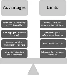
VaR is a risk measurement tool that has advantages and limits. On the one hand, VaR can be seen as a cornerstone in risk management because it is an easy-to-understand method for calculating exposure to risks in single digits. It provides a unified framework for a meaningful, easy to interpret, aggregate measure of risks. For example, a VaR at 99.95% over one year corresponds to one bankruptcy every 200 years. A VaR at 99% over 10 days corresponds to one bankruptcy every 1,000 days. Moreover, VaR uniformly treats different types of risk. For example, the insurance company can calculate two VaRs (one on credit risk and the other on interest rate risk) and can easily compare the results if the level of confidence and the time horizon are the same.

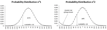
Concerning the limits, VaR is, in practice, often computed under the assumption that the distribution is normal; hence, estimates of tail probabilities can be obtained by estimating the mean and variance of the distribution. Nevertheless, this is often inaccurate. VaR offers little guidance in exploring tail events and is difficult to estimate. This limitation is especially profound for products with an asymmetrical risk profile, such as options and mortgages. In fact, VaR does not capture the subtleties of the probability distribution, especially for tail probabilities. For example, two different probability distributions can give an identical VaR. The two graphs below illustrate this point: in both cases, VaR at 84% is equal to 50, while the probability distribution is different. However, the second distribution hides a greater risk than the first distribution. When the loss exceeds the VaR, there is a high probability that this loss is much greater with the second distribution (approximately 200). In this example, a risk indicator, such as conditional VaR (CVaR) (detailed in section 1.2.2), would be more appropriate.

Figure 1.2. Comparison of two probability distributions on VaR

Moreover, assumptions used for volatilities and correlations, upon which the VaR calculation is highly dependent, can break down during periods of market stress. Indeed, securities that seem uncorrelated during normal times may become extremely highly correlated during market crises.

Furthermore, VaR is not intended to anticipate a crisis because it is only really secure when the underlying distribution is stationary. This assumption is generally not observed in reality; so, to correct this, a stressed VaR, which uses data from 2008 (during the crisis) to be calibrated, was added in a revision of Basel II.

VaR does not capture differences in the liquidity of portfolio assets. Indeed, in the VaR calculation, portfolio assets can be liquidated or covered regardless of their size, with no impact on the market and whether or not there is a crisis. To correct this underestimation of risk, it is possible to calculate a VaR adjusted to liquidity.

Last, but not least, VaR does not take into account wider risk factors such as policy and regulation.

Figure 1.3 shows the advantages and limitations of VaR.

Figure 1.3. Advantages and limitations of VaR

1.2. The use of VaR for insurance companies

Solvency II is based, as are the Basel agreements, on a three-pillar approach:

– Pillar I consists of quantitative requirements (e...

Table of contents

• Cover
• Contents
• Title
• Copyright
• Introduction
• Chapter 1: Use of Value-at-Risk (VaR) Techniques for Solvency II, Basel II and III
• Chapter 2: Classical Value-at-Risk (VaR) Methods
• Chapter 3: VaR Extensions from Gaussian Finance to non-Gaussian Finance
• Chapter 4: New VaR Methods of non-Gaussian Finance
• Chapter 5: non-Gaussian Finance: semi-Markov Models
• Conclusion
• Bibliography
• Index