![]()
PART ONE
The Multiple Linear Regression Model
![]()
CHAPTER ONE
Multiple Linear Regression
1.1 Introduction
1.2 Concepts and Background Material
1.2.1 The Linear Regression Model
1.2.2 Estimation Using Least Squares
1.2.3 Assumptions
1.3 Methodology
1.3.1 Interpreting Regression Coefficients
1.3.2 Measuring the Strength of the Regression Relationship
1.3.3 Hypothesis Tests and Confidence Intervals for β
1.3.4 Fitted Values and Predictions
1.3.5 Checking Assumptions Using Residual Plots
1.4 Example – Estimating Home Prices
1.5 Summary
1.1 Introduction
This is a book about regression modeling, but when we refer to regression models, what do we mean? The regression framework can be characterized in the following way:
1. We have one particular variable that we are interested in understanding or modeling, such as sales of a particular product, sale price of a home, or voting preference of a particular voter. This variable is called the target, response, or dependent variable, and is usually represented by y.
2. We have a set of p other variables that we think might be useful in predicting or modeling the target variable (the price of the product, the competitor’s price, and so on; or the lot size, number of bedrooms, number of bathrooms of the home, and so on; or the gender, age, income, party membership of the voter, and so on). These are called the predicting, or independent variables, and are usually represented by x1, x2, etc.
Typically, a regression analysis is used for one (or more) of three purposes:
1. modeling the relationship between x and y;
2. prediction of the target variable (forecasting);
3. and testing of hypotheses.
In this chapter we introduce the basic multiple linear regression model, and discuss how this model can be used for these three purposes. Specifically, we discuss the interpretations of the estimates of different regression parameters, the assumptions underlying the model, measures of the strength of the relationship between the target and predictor variables, the construction of tests of hypotheses and intervals related to regression parameters, and the checking of assumptions using diagnostic plots.
1.2 Concepts and Background Material
1.2.1 THE LINEAR REGRESSION MODEL
The data consist of n sets of observations {x1i, x2i, … xpi, yi}, which represent a random sample from a larger population. It is assumed that these observations satisfy a linear relationship,
where the β coefficients are unknown parameters, and the εi are random error terms. By a linear model, it is meant that the model is linear in the parameters; a quadratic model,
paradoxically enough, is a linear model, since x and x2 are just versions of x1 and x2.
It is important to recognize that this, or any statistical model, is not viewed as a true representation of reality; rather, the goal is that the model be a useful representation of reality. A model can be used to explore the relationships between variables and make accurate forecasts based on those relationships even if it is not the “truth.” Further, any statistical model is only temporary, representing a provisional version of views about the random process being studied. Models can, and should, change, based on analysis using the current model, selection among several candidate models, the acquisition of new data, and so on. Further, it is often the case that there are several different models that are reasonable representations of reality. Having said this, we will sometimes refer to the “true” model, but this should be understood as referring to the underlying form of the currently hypothesized representation of the regression relationship.
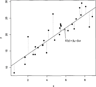
The special case of (1.1) with p = 1 corresponds to the simple regression model, and is consistent with the representation in Figure 1.1. The solid line is the true regression line, the expected value of y given the value of x. The dotted lines are the random errors εi that account for the lack of a perfect association between the predictor and the target variables.
1.2.2 ESTIMATION USING LEAST SQUARES
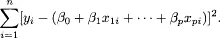
The true regression function represents the expected relationship between the target and the predictor variables, which is unknown. A primary goal of a regression analysis is to estimate this relationship, or equivalently, to estimate the unknown parameters β. This requires a data-based rule, or criterion, that will give a reasonable estimate. The standard approach is least squares regression, where the estimates are chosen to minimize
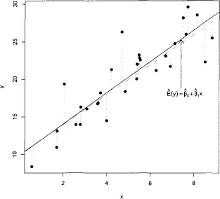
Figure 1.2 gives a graphical representation of least squares that is based on
Figure 1.1. Now the true regression line is represented by the gray line, and the solid black line is the estimated regression line, designed to estimate the (unknown) gray line as closely as possible. For any choice of estimated parameters
, the estimated expected response value given the observed predictor values equals
and is called the
fitted value. The difference between the observed value
yi and the fitted value
i is called the
residual, the set of which are represented by the lengths of the dotted lines in
Figure 1.2. The least squares regression line minimizes the sum of squares of the lengths of the dotted lines; that is, the ordinary least squares (OLS) estimates minimize the sum of squares of the residuals.
In higher dimensions (p > 1) the true and estimated regression relationships correspond to planes (p = 2) or hyperplanes (p ≥ 3), but otherwise the principles are the same. Figure 1.3 illustrates the case with two predictors. The length of each vertical line corresponds to a residual (solid lines refer to positive residuals while dashed lines refer to negative residuals), and the (least squares) plane that goes through the observations is chosen to minimize the...