Breakthrough Strategies for Predicting Any Market

Charting Elliott Wave, Lucas, Fibonacci, Gann, and Time for Profit

Jeff Greenblatt

• Publisher: Wiley
• Year: 2013
• Print ISBN: 9781118585528
• eBook ISBN: 9781118716014
• Edition: 2
• Topic: Business
• Subtopic: Trading
• Index: Business

The revised and updated edition of the book that changed the way you think about trading

In the Second Edition of this groundbreaking book by star trader Jeff Greenblatt, he continues to shares his hard-won lessons on what it takes to be a professional trader, while detailing his proven techniques for mastering market timing. With the help of numerous case studies and charts, Greenblatt develops his original high-probability pattern recognition system which, once mastered, endows its user with a deeper understanding of how the markets really work and boosts the efficiency of any trading methodology.

Following in the footsteps of the great W.D. Gann, Jeff Greenblatt helps investors gain greater precision with any instrument they trade, during any time frame.

• Shows how to combine a variety of technical indicators to pinpoint turning points in the financial markets
• Makes even the most complex subject matter easy to understand with crystal-clear explanations and step-by-step guidance on all concepts, terms, processes, and techniques
• Reveals how to use Elliott Wave Analysis, Fibonacci, candlesticks, and momentum indicators to interpret market movements

Breakthrough Strategies for Predicting Any Market shares fascinating and enlightening personal anecdotes from Jeff Greenblatt's career along with his candid reflection on developing and maintaining the mental discipline of a successful trader.

CHAPTER 1

Underlying Structure of Markets

Welcome to twenty-first century technical analysis! In this work we are going to shatter myths, gore sacred cows, and finally build a better mousetrap. For the past several hundred years, technicians have relied heavily on price and volume studies as the most important factors on a price chart. Don’t get me wrong, these are very important. However they do not give us a complete picture. Time studies are the least understood, yet are a critically important element in technical analysis. For this new edition we are going to include some of the work of W.D. Gann and his most important discovery. So let me say that, while we are in twenty-first century technical analysis, the roots lie in work done 80 to 100 years ago that was ignored by the majority of the trading community. Even today on the three most important media outlets that give us wall-to-wall coverage of markets, the time element is still ignored.

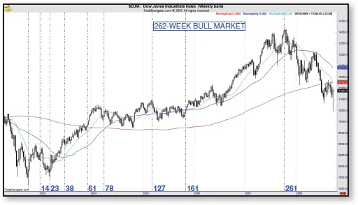
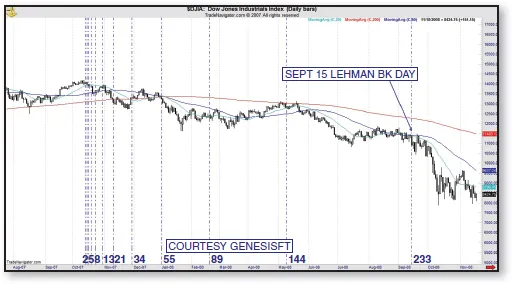
The first edition of this book was released several months before this pattern completed. As early as April 2007 we had been telling our regular readers at the time that a very important pivot was coming in October, as seen in Figure 1.1. The essence of the book was to teach people how to recognize patterns such as this. Had anyone recognized and understood the significance of this market turn they could have taken appropriate action to protect themselves. We revisit this Dow episode later in the book as well because I told people the turn coming in October 2007 could be the most important in that entire decade. I was only partially right. The peak of 2007 turned out to be the most important turn in our generation. It ended a five-year bull market, setting the table for the worst financial crisis since the Great Depression. The timing principles in this book will teach you how to recognize events such as these. One of the most historic was the eye of the storm created by that 262-week high. As we see, the Dow topped on October 11 and 12 in 2007. Exactly 233 trading days later in Figure 1.2, was the Lehman Brothers bankruptcy, which for all practical purposes was the initial acceleration point to the 2008 crash. As it turned out, the NDX/NASDAQ topped out on October 31, 2007, roughly three weeks later.

FIGURE 1.1 Dow Bull Market 2002 to 2007

FIGURE 1.2 Lehman Event

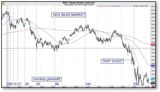
Roughly three weeks after that was the TARP vote in Figure 1.3, which was 233 trading days off the NASDAQ top. It may have been the first time in history that a crash materialized at exactly 233 days off one peak and went into overdrive 233 days off the other peak. If this is really the case it’s because of the unique properties of the 2007 top. Most people don’t know this, but this is the kind of symmetry we are going to teach you how to recognize, along with the opportunities they represent. Also they will help you recognize when an event like this is not materializing. This information was not only valuable to the trading and investing community but the average person who saw his 401(k) decimated as well. If this doesn’t prove the validity of precise market timing windows, nothing ever will.

FIGURE 1.3 TARP Event

Traders comprehend targets based on price and volume very well. However most people have very little idea of the real reason why a trend changes. Do you ever wonder why a chart will hit a certain price target and linger for days until finally one day it drops? Why did it drop on this day as opposed to that day? This area has always been one of the biggest problems for traders. The first edition made a serious attempt to close that gap. This edition takes it a step further. We start here with the symmetry from the greatest crisis in our lifetime and find the market left clues. Hopefully you will continue with an open mind so you can have a greater understanding of why price action behaves the way it does. It is a wonderful world of possibilities. But there has to be a basis for understanding patterns.

There are different methods of technical analysis. Dating back to the 1920s and 1930s, Richard W. Schabacker wrote several books that were based on Dow theory. He hypothesized successfully that certain patterns that showed up in the major averages were also relevant to individual stocks as well. His brother-in-law Robert D. Edwards continued his work. Many in our generation are familiar with the technical work of Edwards and his partner John Magee (Magee ix-xv). Together, they are considered the fathers of modern technical analysis. As we know, technical analysis is a snapshot of market participants’ collective behavior. Since we are dealing with human emotions, these patterns of collective behavior are repeated over and over. They can be recognized and then utilized to anticipate future moves in the markets. These patterns can be further broken down into naturally recurring sets of waves and calculations.

The basic structure of financial markets lies in a catalogue of repeatable patterns uncovered by Ralph Nelson Elliott and refined over the years by other well-known Elliotticians including Robert Prechter Jr. The Wave Principle represents a good pattern-recognition system. These waves are like snowflakes. No two patterns are ever alike, but they all have repeatable tendencies. Inside these waves are universal calculations that are measured in terms of both price and time. These measurements are driven by Fibonacci relationships. Much of the research on the time element is derived from the work of W. D. Gann, who should be considered the founding father of modern time studies. From Gann, modern Fibonacci analysts have done an excellent job of simplifying the methodology so traders can practically use it as an everyday discipline. When you combine Elliott and Gann, you have the capability of taking subjectivity out of Elliott, which is the method’s main criticism. But they are rarely used together.

The Elliott methodology relies heavily on the Fibonacci relationships to the point where one really can’t use one without the other. Since the Wave Principle relies on Fibonacci calculations it would make sense that those who use Fibonacci retracements would recognize patterns in terms of Elliott Waves. The first edition of this book incorporated the time principle into the Fibonacci/Elliott ways of thinking as well as traditional technical analysis. This edition introduces the concept of price and time squaring, Gann’s most important discovery. In this edition we are leaving much of the first edition’s Elliott/Fibonacci work here as many of you are more familiar with it, but taking it one step further and introducing enough Gann you can use now and it won’t take years to figure out. The first edition reintroduced the Lucas series of mathematics. French mathematician Edouard Lucas (1842–1891) discovered this series, which is a derivative of the Fibonacci sequence. Lucas was the guy who gave the Fibonacci sequence its name. It is mentioned briefly in other books. It is here where this series is presented in great detail. The author is certainly not the first to present Lucas to the financial community. However, it has a greater influence on many financial charts in all degrees of trend than many realize, as we will show you, and has been greatly misunderstood and greatly understated. Lucas does not supersede Fibonacci, it complements it. According to the research presented here, you will see how often it does. The purpose of using the time dimension is to gain a very important tool in the pattern-recognition game.

A pilot wouldn’t think to ever take off in a plane that was not equipped with instruments that could fly or land it in bad visibility. As challenging as financial markets are, using technical analysis as a pattern-recognition system without the time dimension is like attempting to land a plane in zero visibility.

Before going on instruments we need to navigate in good weather. Basic navigation of financial markets begins with an understanding of the Wave Principle as one underlying structure of all financial markets. The Wave Principle gives the trader a good start at pattern recognition. Those of you trained in the Edwards and Magee school of technical analysis can compare and contrast the two methodologies. This book uses the Wave Principle only as a guide because it is fairly complex and not totally reliable in real time. It’s a guide because of the subjectivity of the waves. What we’ll cover here in contrast to what is presented in pure orthodox Elliott books is the ability to use the Wave Principle as a GPS. We don’t want to totally rely on the waves as iron trading rules for entry and exit.

When we look at the waves we can have an idea of where we are in a trend. We can also have an idea if we are in the main trend or in a move that technically corrects that trend. Sometimes a correction is so large in relation to the main trend that we really don’t know if the larger trend has changed. This is one of the black holes in the Wave Principle that this book intends to clear up.

There are two basic patterns of waves. The first are known as impulse waves, which is the prevailing larger-degree trend. The other is known as corrective waves, which move counter to the main trend. Each has their own distinctive set of characteristics. In this chapter I will only cover the basics as a review of materials you may have read elsewhere. Later on, I will show you how to recognize an impulse or corrective wave by exclusively understanding the number sequences in all of these waves.

■ Impulse Waves

Impulse waves have their own unique characteristics. The larger prevailing trend is considered to be an impulse wave and you can recognize them as they move in a five-wave sequence. They can also move in a 9- or 13-wave pattern. There are only three iron laws of impulse waves according to Prechter (30).

1. Wave three is never the shortest wave.

2. Wave two never retraces more than 99 percent of wave one.

3. Wave four does not overlap the territory of wave one.

Let’s clear up some of the confusion surrounding these rules. From my experience in dealing with the Elliott community over the past few years, some think the third wave is always the largest wave. This is simply not the case. Generally speaking, the tendency is for wave three to be the largest wave, but the rule is it can’t be the shortest wave. If you are counting waves and the middle wave is the smallest, something else is going on. That particular wave might be an extension of the first wave, but it isn’t a third wave.

The other controversy surrounds fourth waves. According to some in the Elliott community, they do not allow for any overlap of the first and fourth waves, but I’ve seen many instances of where the fourth wave touches, grazes, or slightly overlaps wave one. I think you need to apply common sense to the situation. If you have a fourth wave that makes an obvious violation into first-wave territory, it isn’t a fourth wave. If you’ve had a first wave, a retracement second wave, a third that makes a decent advance, and then you have a pullback that grazes first-wave territory before turning up, I think you can make a case for it being a fourth wave.

Another characteristic of impulse waves is the Rule of Alternation. This is not an iron law but rather a guideline. The Rule of Alternation suggests that if the second wave retracement takes the form of a sharp, the fourth wave is likely to be a flat correction. Other ways this rule manifests itself is when the first wave is the largest wave, the fifth wave will be the smallest. In a larger move, if one set of five waves has the third wave as the extension, the next round will either have the first or fifth wave as the extended wave (Prechter 61).

Extensions are another important characteristic of impulse waves. This means that of waves one, three, or five, one will be considerably larger than the other two. Extensions are hard to count while they are in progress, and the exact count is not readily apparent until late in the move. The time cycles clear up much of the confusion and allow the trader or analyst a better roadmap to determine where we are in the bigger scheme of things more easily.

There is a set of common relationships in an impulse sequence that is Fibonacci based. The most common tendency is for the third wave to be the extended wave and many times it will measure 1.618 or 2.618 times the length of wave one as measured from the bottom of wave two (Prechter 125-138). In lower probability cases, the third wave may even measure 4.23 times the length of wave one.

When the third wave is the extended wave, the tendency is for waves one and five to have a 0.618/1.618 relationship to each other. In rare cases, the fifth wave can be a 2.618 extension of wave one. Recently, we had a situation in the XAU where wave five was a 2.618 extension of wave one and wave three was not the shortest wave.

When a fifth wave extends, the most common relationship is it measures 1.618 times the length of waves one through three, with wave one being the smallest wave. When wave one extends, it will usually measure 1.618 times the length of waves three through five, with wave five being the smallest wave.

In rare cases we can have a double extension where waves three and five are both twin 4.23 extensions of the first wave.

The best way to recognize an extended wave is to observe how the progression begins. Once we get a new trend we’ll have a first wave up, a retracement, and another leg up. If the second retracement violates into the territory of the very first wave in the sequence, we know by the iron law of fourth waves, that this can’t be a fourth wave. It must be the start of an extension or larger move. How do we know that it is not a corrective move? Watch the volume patterns. At all times we will use other indicators to confirm a wave count. If we are in an uptrend, the down days compared to the up days will be lower volume on average. For instance, if we’ve been through a long down trend where sentiment became unusually negative, the trend going in the new direction will start to build decent volume days and the pullbacks will be of lighter volume. A lighter volume wave that slightly overlaps a first wave up is likely to be corrective, counter to the new trend and part of an extension going in the new direction. The time dimension will also give us a good clue as to the underlying direction and I’ll cover that in a later chapter.

■ Corrective Waves

Corrective waves have their own unique set of characteristics that differentiate them from impulse waves. A wave is corrective when it moves counter to the trend. There are two types of corrective waves. One family consists of sharp corrections and the other family is considered flat corrections. You may consider triangles to be another subset, but technically they are part of the flat family.

Sharp corrections normally fall into a five-three-five pattern of waves. They are labeled differently from impulse waves and use letters as opposed to numbers. An ABC correction will contain five small waves moving counter to the trend, followed by a small sideways or triangle correction, followed by five more waves. The way to recognize these waves is they violate the overlap rule where the fourth wave falls deep into the territory of the first wave. The best way to recognize a sharp correction is they are distinguished by being very choppy. If you don’t understand waves at all and have no real plan to do so, the best way to understand corrective moves is by their choppiness or lack of structure. Corrective waves are also characterized by an average lower volume than the prevailing larger-degree trend moving in the other direction. How do you know you are in a correction? Let’s say we are in a bear market and begin a bounce. If the up days are on light volume it’s bound to fail. It can be as simple as that.

Sharp corrections retrace either 38 percent, 50 percent, 61 percent, 78 percent, or 88.6 percent. In rare cases they will retrace 23 percent. Several years back a study was done by Rich Swannell, an Australian Elliottician. He took millions of retracements in all degrees of trend and found that 60 percent of second wave retracements fell under the bell curve between the 25 to 70 percent retracement level (34-35). This adds to the complexity, since 40 percent of the time we will have some other retracement such as the 14.6 percent or even the 88.6 percent. How one definitively defines a second wave in an impulse or a B wave in a corrective, I’m not sure.

We derive the 88.6 level because it is the square root of the 0.786 retracement level. However, moves will stop short of a full retest right on the 88.6 percent marker. For most common retracement relationships, the following happens. An impulse move in one direction will occur, and when it comes time to retrace, the first leg will retrace 38 percent counter to the trend. This would be an A wave or the first part of an ABC. A small B wave commences, and finally the C wave kicks in ...

Table of contents

• Cover
• Half Title Page
• Title Page
• Copyright
• Dedication
• Contents
• Foreword
• Preface
• Acknowledgments
• Chapter 1: Underlying Structure of Markets
• Chapter 2: Elliott Waves
• Chapter 3: Rotation
• Chapter 4: Candlesticks
• Chapter 5: Divergences
• Chapter 6: Volume Studies and Moving Averages
• Chapter 7: Fibonacci Price Projections
• Chapter 8: Advanced Projection Techniques
• Chapter 9: Forex
• Chapter 10: Squaring of Price and Time
• Chapter 11: Andrews Pitchforks Crash Course
• Chapter 12: Square of 9
• Chapter 13: Psychology
• Chapter 14: Market Psychology/Sentiment
• Chapter 15: Building the Bridge
• Chapter 16: Conclusion
• Bibliography
• Author’s Disclaimer
• About the Author
• Index