![]()
Chapter 1
General Principles of MRI
Bich-Thuy Doan,1 Sandra Meme,2 and Jean-Claude Beloeil3
1CNRS, Chimie-Paristech, Université Paris Descartes, Paris, France
2Centre de Biophysique Moléculaire, CNRS, Orléans, France
1.1 Introduction
Magnetic Resonance Imaging (MRI) derives directly from the phenomenon of Nuclear Magnetic Resonance (NMR [1–4]), which is widely used by chemists to determine molecular structure. The word “nuclear” was dropped in the switch to imaging to avoid alarming patients as NMR has nothing to do with radioactivity. This book is intended mainly for chemists, who are generally familiar with the NMR spectra. After a brief overview of the technique explaining the notion of relaxation time and saturation transfer used in MRI, we will describe localization techniques, which are less well-known in chemistry. The purpose of this short chapter is not to provide a complete theory of MRI [5–8], but to understand the rest of the book concerning the action of contrast agents. We will not go into the theoretical background of the phenomena, and while it is important to have some understanding of quantum mechanics, it is not our purpose to develop this aspect. This is a “nuts and bolts” description of MRI. Whenever possible, we refer to chemists' knowledge of NMR (for example, “2D NMR”).
1.2 Theoretical basis of NMR
1.2.1 Short description of NMR
In most cases, MRI focuses on one type of atomic nucleus, that of hydrogen in H2O. We will therefore only use this nucleus, termed the “1H proton.”
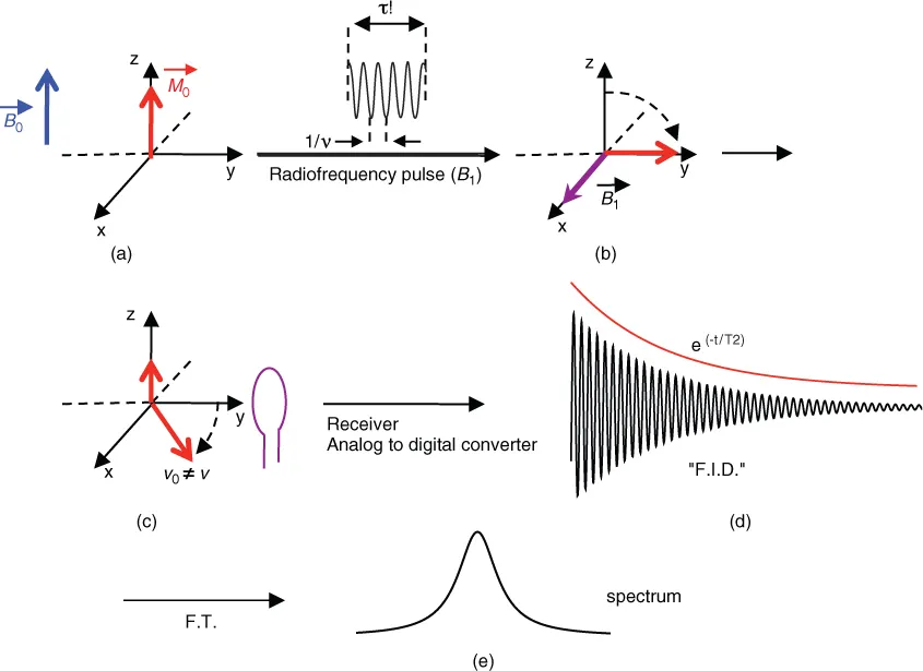
The physical phenomenon of NMR lies at the boundary between “conventional” and “quantum” treatment due to the small transition energies involved. Traditionally, the 1H proton can be considered as a charged sphere rotating with a magnetic moment and collinear angular momentum (in quantum mechanics, these two entities are quantified as magnetic quantum number and spin quantum number (or spin)). Like a spinning top precessing in the Earth's gravitational field, the nucleus 1H precesses in the static magnetic field B0 of the spectrometer magnet. This precession will occur at a frequency (ν0) dictated by the nature of the nucleus and the strength of the magnetic field of the magnet (ν0 = −(γ/2π)B0) (Larmor frequency). There are two possible precessions (parallel and antiparallel to B0) corresponding to two energy states in the presence of a strong magnetic field. According to the Boltzmann equation, there are more 1H protons in the lower level (parallel to B0) than in the upper level. There will be total magnetization (M0) of the sample, parallel to B0 (by definition, the z axis) (Figure 1.1). The whole process of obtaining a spectrum is summarized in Figure 1.1.
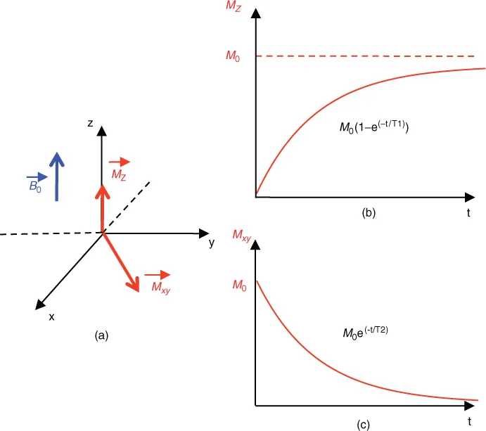
In an NMR experiment, the sample is subjected to the action of an oscillating electromagnetic field (B1) (frequency: ν1) perpendicular to B0 (Figure 1.1); if we place ourselves within a rotating frame around the z axis at frequency ν1 (ν1 close to ν0), it is as if the magnetization M0 precesses around the magnetic field B1, which is stationary within this frame. The duration of the B1 field (pulse) is calculated for a M0 tilt of 90°, or, more generally, of a flip angle α. At the end of the RF pulse, the system then returns to equilibrium, the magnetization in the xy plane decreases exponentially with time constant T2, and the magnetization rises exponentially on axis z with a time constant T1 (T2 < T1) (Figure 1.2). If we put a receiver coil in the xy plane, an electric current is induced in the coil and a signal is obtained after analog/digital conversion into a damped sinusoid called Free Induction Decay (FID).
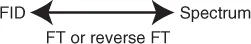
This signal corresponds to a temporal frequency. The Fourier transform (FT) of this signal (Figure 1.1) provides a spectrum of frequencies contained in the signal; in this case just one because we are only interested in H2O. The signal intensity is proportional to the quantity of 1H protons and therefore the amount of H2O in the sample. In NMR, it is observed that we have a temporal frequency (FID) and that the FID and spectrum are a Fourier pair (Scheme 1.1).
1.2.2 Relaxation times
Unlike other spectroscopic techniques, the energy difference between the excited state and steady state is too low to allow spontaneous relaxation, and therefore relaxation needs to be stimulated. The longitudinal relaxation time T1 (Figure 1.2b) is characteristic of the return to equilibrium of the magnetization (Figure 1.2a) along z (Mz = M0 (1−e−t/T1)); this phenomenon corresponds to the enthalpic interaction of the excited nucleus with its environment, and in particular with the magnetic active agents of this environment (1H protons, unpaired electrons e−). The movement of nuclear magnetic moments of other molecules (or unpaired e−) creates a distribution of frequencies within which one can find the resonance frequency of the excited nucleus, and a stimulated relaxation may then occur. Therefore, for this mechanism to work, there must be a movement of the molecules (Brownian motion). T1 relaxation time will depend on the mobility of these entities and therefore on the viscosity of the environment.
The T2 transversal relaxation time is characteristic of the disappearance of the signal in the xy plane (Figure 1.2c). It is an entropy phenomenon that corresponds to spin dephasing in the xy plane. T2 is always below T1. A parameter often used in MRI is the relaxation time T2*, which contains both T2 and the contribution of all magnetic field inhomogeneities and therefore those that are characteristic of the sample. T2* is thus linked to specific properties of the tissue under study and is very useful in medical MRI.
1.2.3 Saturation transfer
The saturation phenomenon is used in NMR to identify hydrogens in conformational or chemical exchange. It is easy to obtain saturati...