Mathematical Foundations of Image Processing and Analysis 1

Jean-Charles Pinoli

• Publisher: Wiley-ISTE
• Year: 2014
• Print ISBN: 9781848215467
• eBook ISBN: 9781118649121
• Edition: 1
• Topic: Technology & Engineering
• Subtopic: Signals & Signal Processing
• Index: Technology & Engineering

Image processing and image analysis are typically important fields in information science and technology. By "image processing", we generally understand all kinds of operation performed on images (or sequences of images) in order to increase their quality, restore their original content, emphasize some particular aspect of the information or optimize their transmission, or to perform radiometric and/or spatial analysis. By "image analysis" we understand, however, all kinds of operation performed on images (or sequences of images) in order to extract qualitative or quantitative data, perform measurements and apply statistical analysis. Whereas there are nowadays many books dealing with image processing, only a small number deal with image analysis. The methods and techniques involved in these fields of course have a wide range of applications in our daily world: industrial vision, material imaging, medical imaging, biological imaging, multimedia applications, satellite imaging, quality control, traffic control, and so on

PART 1

An Overview of Image Processing and Analysis (IPA)

1

Gray-Tone Images

In this textbook, the term image will have a physical meaning and will refer to a one-, two- or threedimensional (3D), continuous or discrete (including the digital form) radiometric spatial distribution of light (or another radiation) intensities.

1.1. Intensity images, pixels and gray tones

Radiometric images are spatially defined on pixels (contraction of “picture elements”) with intensity values called gray tones. Such images are often abusively called “black and white” images in the common language (panchromatic images is better suited and sometimes used in relation to the visible light and the human eye) [ALL 10; Original 1st ed., 1890]. In this book, they will be naturally designated as gray-tone images. Color images (e.g. three colors according to the human visual perception), multispectral images (e.g. four or five colors as in satellite imagery) [LEE 05] [PET 10; p. 665] and hyperspectral images (i.e. numerous almost monochromatic channels) [CHA 03b] will not be discussed because they require specific frameworks and approaches, still subject to particular mathematical research works.

The term illumination designates the incident light (or another radiation, such as an electromagnetic or nuclear radiation, e.g. gamma rays and X-rays) [DAI 74, HEN 02, BAR 04, HOR 06].

There exist a lot of imaging modalities, in particular for materials investigation, and in biological and medical imaging, but also in many other scientific, engineering or technical fields, as well for professional and personal purposes (e.g. magnetic resonance imaging (MRI), positron emission tomography (PET), scanning electron microscopy (SEM), transmission electron microscopy (TEM) and ultrasound imaging (US)).

The term imaging, although wider than the terms “image processing” and “image analysis”, as it also includes “image acquisition” and “image visualization” aspects (see section I.1), will be employed with a general meaning in this book.

1.2. Scene, objects, context, foreground and background

The term scene designates generically everything that is observed, i.e. a particular physical environment, and takes different names according to the addressed situations and concerned users: (1) sample (e.g. in metallography or histology), (2) raw or manufactured component (e.g. in industrial inspection), (3) body or organ (e.g. in medical imaging), (4) specimen (e.g. in biology or zoology), etc.

An image is an observation of a scene, which is most often a partial and incomplete view of it, called field of view (FoV). The observed scene, depending on (1) the light (e.g. visible, infrared, ultraviolet or X-rays light) or (2) another radiation (e.g. electronic) constituting the illumination (see section 1.1), (3) the nature of its interaction with this illumination (e.g. simple reflection or fluorescence) and (4) the type of collected images (e.g. by transmission or reflection), will be investigated through a field of observation (i.e. FoV) corresponding to a width and length for two-dimensional (2D) imaging, as well as a depth of field (DoF) for 3D imaging. It is a major difficulty in imaging.

In a scene, there are objects located in a context, generally called the “background”. Depending on the addressed situation or the application issue, the context is also called (1) ambient space (e.g. in Geometry or Physics), (2) matrix (e.g. in Geology, or in Materials Sciences and Engineering), (3) medium (e.g. in Biology, or Chemical Sciences and Engineering), etc., while a class of similar objects will be called (1) phase (e.g. in Physics), or (2) population (e.g. in Biology, or Chemical Sciences and Engineering), etc. The term “object” is thus very general.

Therefore, an image ‘ideally’ includes background pixels, corresponding to the context, and foreground pixels, corresponding to the objects, or more often only to parts of objects. The term ‘ideal’ expresses the fact that in reality some pixels or groups of pixels can be wrongly considered as belonging to the other category. This is another major difficulty in imaging.

1.3. Simple intensity image formation process models

The purpose of this section is to present several image formation process models and laws that form the basis of the main imaging processes.

1.3.1. The multiplicative image formation process model

The basic nature of an intensity image, denoted by f, may be considered as being characterized by two components [OPP 68, HUA 71] [GON 87; section 2.2; 1st ed., 1977]. One component is the amount of light (or another radiation) incident on the scene being observed, while the other is the amount of light (or another radiation) reflected (or transmitted) by the scene. These two components are appropriately called the illumination and reflectance (or transmittance), and are denoted by i and r (or t), respectively. These two functions combine as a product to form an intensity image f, which is given at spatial location x by [OPP 68, STO 72, PIN 97a]:

[1.1]

[1.2]

where 0 < i(x) < +∞ and 0 ≤ r(x) ≤ 1, and “·” is the standard product operation.

1.3.1.1. Lambert’s reflection cosine law

Lambert’s reflection cosine law [LAM 60] states that the apparent brightness of a Lambertian surface is proportional to the cosine of the angle between the surface normal and the direction of the incident light at spatial location x [PRA 07; p. 55.; 1st ed., 1978] [PED 93] [BRO 08; p. 273]:

[1.3]

where f_r(x) is the intensity of the diffusely reflected light (i.e. surface brightness), i(x) is the intensity of the incoming light and θ(x) is the angle between the direction of the two vectors (assuming that f_r(x) = 0 when the cosine takes on negative values).

The reflected intensity will be the highest if the surface is perpendicular to the direction of the light, and the lowest if the surface runs parallel with the direction of the light.

The reflection coefficient, reflection ratio, denoted r(x) (0 ≤ r(x) ≤ 1), given by [BRO 08; p. 273]:

[1.4]

is called the albedo [LAM 60] (from the Latin term albedo which means “whiteness”), and is the ratio of reflected radiation from the surface to the incident radiation upon it.

In general, the albedo depends on the directional distribution of incident radiation, except for Lambertian surfaces which scatter radiation in all directions according to a cosine function and therefore have an albedo that is independent of the incident radiation distribution.

1.3.1.2. Bouguer–Beer–Lambert’s attenuation law

In Optics, Bouguer–Beer–Lambert’s attenuation law [BOU 29, LAM 60, BEE 52] relates the absorption of light (or another radiation) to the properties of the material through which the light (or another radiation) travels.

Bouguer–Beer–Lambert’s attenuation law can be expressed at spatial location x by [HUN 75] [ATK 10; 1st ed., 1978]:

[1.5]

where f_t(x) is the transmitted intensity, i(x) is the incident intensity, C_BBL is an attenuation coefficient (i.e. a strictly positive real number) that depends on the material and z(x) is the traveled thickness through the material.

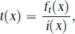
The ratio of intensities is a real-number value, denoted t(x), called the transmittance ratio (0 ≤ t ≤ 1):

[1.6]

assuming that the incident intensity is not zero.

1.3.1.3. Hounsfield’s X-ray unit

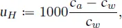
In X-ray imaging, Hounsfield unit (HU) is defined by [FEE 10]:

[1.7]

where c_a and c_w are the attenuation coefficients of the material and the (distilled) water (under specific conditions, i.e. standard pressure and temperature), respectively.

1.3.1.4. Hurter–Driffield’s photographic recording law

The Hurter–Driffield photographic recording law [HUR 90, HUR 98], which was stated in the 1870s for photographic film recording, relates the film density (i.e. the logarithm of opacity) versus the logarithm of the total exposure called the characteristic Hurter–Driffield’s curve. The overall shape of such a curve is a bit like an “S” slanted so that its base (the ‘fog’ region) and top (the saturation region) are horizontal (i.e. a sigmoid curve [SEG 07]), and with a central region which approximates to a straight line. The slope of this ‘straight-line’ portion is called the HD-gamma [HUN 75].

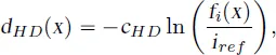
Within this portion, Hurter–Driffield’s photographic recording law can be expressed at spatial location x by [HUN 75] [PRA 07; p. 356, 1st ed., 1978] [CAR 00]:

[1.8]

where d_HD(x) is the optical density, f_i(x) is the incident intensity, i_ref is the reference intensity value (i_ref ≥ f(x)) and c_HD is the HD-gamma proportionality constant that depends on the units used.

1.3.2. The main human brightness perception laws

Subjective or perceptual brightness is an attribute of (human) visual perception in which a scene appears to be reflecting or transmitting light. This is a subjective attribute of a scene being observed.

The specialized literature describing human brightness response to stimulus intensity includes many uncorrelated results due to the various viewpoints and focus interests of researchers from different scientific disciplines [XIE 89, KRU 89, KRU 91. Several human brightness perception laws have been studied and reported, e.g. Weber’s law, Fechner’s law, deVries-Rose’s law, Stevens’s law and Naka–Rushton’s electrophysiological law.

1.3.2.1. Weber’s brightness perception law

The response to light intensity by the human visual system has been known to be nonlinear since the mid-19th Century, when the psychophysician E.H. Weber [WEB 46] established the now so-called “Weber’s visual law”. He argued that the human visual detection depends on the ratio, rather than the difference, between two incident light intensity values f and f + df, where df is the so-called just noticeable difference (JND), also called the least perceptible difference [JUD 32], which is the amount of light necessary to add to a visual test field of constant intensity value f such that it can be discriminated from the reference light field of constant intensity value f [GOR 89; p. 17] [WAT 91].

Weber’s brightness perception law is expressed as [GOR 89; p. 18]:

[1.9]

where f and f + df are two just noticeable incident light intensities (i.e. the magnitudes of the physical stimuli), and c_W is a real-number constant called Bouguer-Weber’s constant that has been found to be near 0.025 for retinal rods [COR 65].

1.3.2.2. Fechner’s brightness perception law

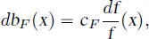
A few years after Weber, G. Fechner [FEC 60] (Weber’s student) explained the nonlinearity of the human visual perception as follows: in order to produce incremental arithmetic steps in sensation, the light intensity must grow geometrically. He proposed the following relationship between the incident light intensity f (the so-called stimulus) and the brightness b_F (the so-called sensation):

[1.10]

where df is the increment of incident light that produces the increment db_F of visual sensation (brightness), and c_F is a real-number constant that depends on the units used.

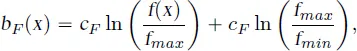
Fechner’s brightness perception law can then be expressed as [GOR 89; p. 17]:

[1.11]

where f(x) is the incident light intensity (i.e. the magnitude of the physical stimulus), b_F(x) is the brightness (i.e. the subjective magnitude of the sensation evoked by the stimulus), f_min is the absolute threshold [COR 70; Chapters 2 and 4] [GOR 89; p. 15] of the human visual system, which is known to be very close to the physical complete darkness [PIR 67, ZUI 83], and c_F is a strictly positive real-number proportionality constant that depends on the units used.

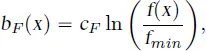
Fechner’s brightness perception law can be equivalently expressed as [PIN 97b]:

[1.12]

where f_max is the upper threshold (or glare limit) of the Human Vision [GON 87; p. 39, 1st ed., 1977] [LEV 00].

1.3.2.3. Stevens’s brightness perception law

In the 1950s, S.S. Stevens [STE 57b, STE 57a, STE 64] proposed a power law for describing the relationship between the magnitude of a physical stimulus and its perceived intensity or strength.

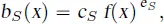
The general form of Stevens’s brightness perception law is [GOR 89; p. 30]:

[1.13]

where f(x) is the incident light intensity (i.e. the magnitude of the physical stimulus), b_S(x) is the brightness (i.e. the subjective magnitude of the sensation evoked by the stimulus), c_S is a strictly positive real-number proportionality constant that depends on the units used and e_S is an exponent, called Stev...

Table of contents

• Cover
• Contents
• Dedication Page
• Title Page
• Copyright Page
• Preface
• Introduction
• Elements of Mathematical Terminology
• PART 1: An Overview of Image Processing and Analysis (Ipa)
• PART 2: Basic Mathematical Reminders for Gray-tone and Binary Image Processing and Analysis
• PART 3: The Main Mathematical Notions for the Spatial and Tonal Domains
• PART 4: Ten Main Functional Frameworks for Gray Tone Images
• Appendices
• Tables of Notations and Symbols
• Table of Acronyms
• Table of Latin Phrases
• Bibliography
• Index of Authors
• Index of Subjects