![]()
CHAPTER 1
Thermal, Mechanical, Quantum, and Analytical Sensors
1-0 INTRODUCTION
Automated laboratory systems, manufacturing process controls, analytical instrumentation, and aerospace systems all would have diminished capabilities without the availability of contemporary computer-integrated data systems with multisensor information structures. This text accordingly develops supporting error models that enable a unified performance evaluation for the design and analysis of linear and digital instrumentation systems with the goal of compatibility of integration with enterprise quality requirements. These methods then serve as a quantitative framework supporting the design of high-performance automation systems.
This chapter specifically describes the front-end electrical sensor devices for a broad range of applications from industrial processes to scientific measurements. Examples include environmental sensors for temperature, pressure, level, and flow; optical sensors for measurements beyond apparatus boundaries, including spectrometers for chemical analytes; and material and biomedical assays sensed by microwave microscopy. It is notable that owing to advancements in higher attribution sensors they are increasingly being substituted for process models in many applications.
1-1 INSTRUMENTATION ERROR INTERPRETATION
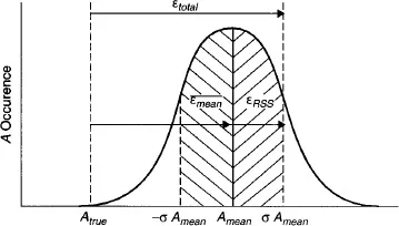
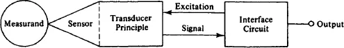
Measured and modeled electronic device, circuit, and system error parameters are defined in this text for combination into a quantitative end-to-end instrumentation performance representation for computer-centered measurement and control systems. It is therefore axiomatic that the integration and optimization of these systems may be achieved by design realizations that provide total error minimization. Total error is graphically described in Figure 1-1, and analytically expressed by Equation (1-1), as a composite of mean error contributions (barred quantities) plus the root-sum-square (RSS) of systematic and random uncertainties. Total error thus constitutes the deviation of a sensor-based measurement from its absolute true value, which is traceable to a standard value harbored by the National Institute of Standards and Technology (NIST). This error is traditionally expressed as 0–100% of full scale (%FS), where the RSS component represents a one-standard-deviation confidence interval, and accuracy is defined as the complement of error (100% − εtotal). Figure 1-2 illustrates generic sensor elements and the definitions describe relevant terms:
| Accuracy: | The closeness with which a measurement approaches the true value of a measurand, usually expressed as a percent of full scale |
| Error: | The deviation of a measurement from the true value of a measurand, usually expressed as a percent of full scale |
| Tolerance: | Allowable deviation about a reference of interest |
| Precision: | An expression of a measurement over some span described by the number of significant figures available |
| Resolution: | An expression of the smallest quantity to which a quantity can be represented |
| Span: | An expression of the extent of a measurement between any two limits |
| Range: | An expression of the total extent of measurement values |
| Linearity: | Variation in the error of a measurement with respect to a specified span of the measurand |
| Repeatability: | Variation in the performance of the same measurement |
| Stability: | Variation in a measurement value with respect to a specified time interval |
Technology has advanced significantly as a consequence of sensor development. Sensor nonlinearity is a common source of error that can be minimized by means of multipoint calibration. Practical implementation often requires the synthesis of a linearized sensor that achieves the best asymptotic approximation to the true value over a measurement range of interest.
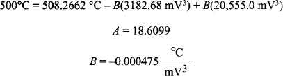
The cubic function of
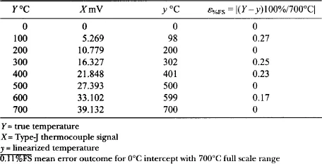
Equation (1-2) is an effective linearizing equation demonstrated over the full 700°C range of a commonly applied Type-J thermocouple, which is tabulated in
Table 1-1. Solution of the
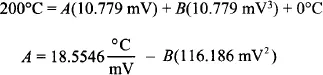
A and
B coefficients at judiciously spaced temperature values defines the linearizing equation with a 0°C intercept. Evaluation at linearized 100°C intervals throughout the thermocouple range reveals temperature values nominally within 1°C of their true temperatures, which correspond to typical errors of 0.25%FS. It is also useful to express the average of discrete errors over the sensor range, obtaining a mean error value of
FS for the Type-J thermocouple. This example illustrates a design goal proffered throughout this text of not exceeding one-tenth percent error for any contributing system component. Extended polynomials permit further reduction in linearized sensor error while incurring increased computational burden, where a fifth-order equation can beneficially provide linearization to 0.1 °C, corresponding to
FS mean error.
Table 1-1. Sensor cubic linearization
Coefficient for 10.779 mV at 200°C:
Coefficient for 27.393 mV at 500°C:
1-2 TEMPERATURE SENSORS
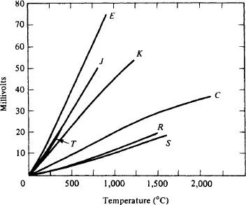
Thermocouples are widely used temperature sensors because of their ruggedness and broad temperature range. Two dissimilar metals are used in the Seebeck-effect temperature-to-emf junction with transfer relationships described by Figure 1-3. Proper operation requires the use of a thermocouple reference junction in series with the measurement junction to polarize the direction of current flow and maximize the measurement emf. Omission of the reference junction introduces an uncertainty evident as a lack of measurement repeatability equal to the ambient temperature.
An electronic reference junction that does not require an isolated supply can be realized with an Analog Devices AD590 temperature sensor as shown in Figure 4-5. This reference junction usually is attached to an input terminal barrier strip in order to track the thermocouple-to-copper circuit connection thermally. The error signal is ...