![]()
Section VI
FOUNDATIONAL ISSUES
![]()
Chapter 20
PROBABILISTIC MODELING WITH BAYESIAN NETWORKS
RICHARD E. NEAPOLITAN
SCOTT MORRIS
20.1. INTRODUCTION
Given a set of random variables, probabilistic modeling consists of acquiring properties of a joint probability distribution of the variables and thereby representing that distribution. These properties can be very important because they often enable us to succinctly represent a distribution and to do inference with the variables. For example, we may be able to concisely represent a joint probability distribution of diseases and manifestations in a medical application and, using this representation, compute the probability that a patient has certain diseases given the patient has some manifestations. First, Section 20.2 gives a brief philosophical overview of the notion of a probability as a relative frequency, which probabilistic modeling using data presupposes. Then, Section 20.3 introduces Bayesian networks and Bayesian network models (also called directed acyclic graph [DAG] models). Next, Section 20.4 discusses learning DAG models. Finally, Section 20.5 shows applications of learning DAG models.
20.2. PHILOSOPHICAL BACKGROUND
The focus of this chapter is on learning DAG models from data. The enterprise of learning something about a probability distribution from data relies on the notion of a probability as a relative frequency. So we first review the relative frequency approach to probability, and then we discuss its relationship to another approach to probability, called subjective or Bayesian.
20.2.1. The Relative Frequency Approach to Probability
In 1919, Richard von Mises developed the relative frequency approach to probability, which concerns repeatable identical experiments. First we describe relative frequencies, and then we discuss how we can learn something about them from data.
20.2.1.1. Relative Frequencies
von Mises (1928/1957) formalized the notion of repeatable identical experiments as follows:
The term is “the collective,” and it denotes a sequence of uniform events or processes which differ by certain observable attributes, say colours, numbers, or anything else. (p. 12, emphasis added)
The classical example of a collective is an infinite sequence of tosses of the same coin. Each time we toss the coin, our knowledge about the conditions of the toss is the same (assuming we do not sometimes “cheat” by, for example, holding it close to the ground and trying to flip it just once). Of course, something is different in the tosses (e.g., the distance from the ground, the torque we put on the coin, etc.) because otherwise, the coin would always land heads or always land tails. But we are not aware of these differences. Our knowledge concerning the conditions of the experiment is always the same. von Mises (1928/1957) argued that, in such repeated experiments, the fraction of occurrence of each outcome approaches a limit, and he called this limit the probability of the outcome. It has become standard to call this limit a relative frequency and to use the term probability in a more general sense.
Note that the collective (infinite sequence) only exists in theory. We never will toss the coin indefinitely. Rather, the theory assumes that there is a propensity for the coin to land heads, and as the number of tosses approaches infinity, the fraction of heads approaches this propensity. For example, if m is the number of times we toss the coin, Sm is the number of heads, and p is the true value of the propensity for the coin to land heads, then
Because the propensity is a physical property of the coin, it is also called a physical probability. In 1946, J. E. Kerrich conducted many experiments using games of chance (e.g., coin tosses) indicating that the fraction does appear to approach a limit.
Note further that a collective is only defined relative to a random process, which, in the von Mises theory, is defined to be a repeatable experiment for which the infinite sequence of outcomes is assumed to be a random sequence. Intuitively, a random sequence is one that shows no regularity or pattern. For example, the finite binary sequence “1011101100” appears random, whereas the sequence “1010101010” does not because it has the pattern “10” repeated five times. There is evidence that experiments such as coin tossing and dice throwing are indeed random processes. Namely, Iversen, Longcor, Mosteller, Gilbert, and Youtz (1971) ran many experiments with dice indicating that the sequence of outcomes is random. It is believed that unbiased sampling also yields a random sequence and is therefore a random process. See van Lambalgen (1987) for a thorough discussion of this matter, including a formal definition of random sequence. Neapolitan (1990) provides a more intuitive, less mathematical treatment. We close here with an example of a nonrandom process. One of the authors prefers to exercise at his health club on Tuesday, Thursday, and Saturday. However, if he misses a day, he usually makes up for it the following day. If we track the days he exercises, we will find a pattern because the process is not random.
Under the assumption that the fraction approaches a limit and that a random sequence is generated, in 1928, von Mises was able to derive the rules of probability theory and the result that the trials are probabilistically independent. In terms of relative frequencies, what does it mean for the trials to be independent? The following example illustrates what it means. Suppose we develop many sequences of length 20 (or any other number), where each sequence represents the result of 20 coin tosses. Then we separate the set of all these sequences into disjoint subsets such that the sequences in each subset all have the same outcome on the first 19 tosses. Independence means that the fraction of heads on the 20th toss is the same in all the subsets (in the limit).
A common way to define probability in applications such as games of chance is to assign the same probability to all possible elemental outcomes. For example, in the draw of the top card from an ordinary deck of cards, each elemental outcome is assigned a probability of 1/52 because there are 52 different cards. Such probabilities are called ratios. We say we are using the principle of indifference (a term popularized by J. M. Keynes in 1921/1948) when we assign probabilities this way. The probability of a set of elemental outcomes is the sum of the probabilities of the outcomes in the set. For example, the probability of a king is 4/52 because there are four kings. How are relative frequencies related to ratios? Intuitively, we would expect that if, for example, we repeatedly shuffled a deck of cards and drew the top card, the ace of spades would come up about 1 out of every 52 times. In the experiment performed by J. E. Kerrich in 1946 (discussed above), the principle of indifference seemed to apply, and the limit was indeed the value obtained via the principle of indifference.
20.2.1.2. Sampling
Sampling techniques estimate a relative frequency for a given collective from a finite set of observations. In accordance with standard statistical practice, we use the term random sample (or simply sample) to denote the set of observations, and we call a collective a population. Note the difference between a collective and a finite population. There are currently a finite number of smokers in the world. The fraction of them with lung cancer is the probability (in the sense of a ratio) of a current smoker having lung cancer. The propensity (relative frequency) of a smoker having lung cancer may not be exactly equal to this ratio. Rather, the ratio is just an estimate of that propensity. When doing statistical inference, we sometimes want to estimate the ratio in a finite population from a sample of the population, and other times we want to estimate a propensity from a finite sequence of observations. For example, TV raters ordinarily want to estimate the actual fraction of people in a nation watching a show from a sample of those people. On the other hand, medical scientists want to estimate the propensity with which smokers have lung cancer from a finite sequence of smokers. One can create a collective from a finite population by returning a sampled item back to the population before sampling the next item. This is called sampling with replacement. In practice, it is rarely done, but ordinarily, the finite population is so large that statisticians make the simplifying assumption that sampling is done with replacement. That is, they do not replace the item, but they still assume the finite population is unchanged for the next item sampled. In this chapter, we are always concerned with propensities rather than current ratios, so this simplifying assumption does not concern us.
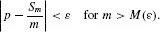
Estimating a relative frequency from a sample seems straightforward. That is, we simply use Sm/m as our estimate, where m is the number of trials and Sm is the number of successes. However, there is a problem in determining our confidence in the estimate. That is, the von Mises theory only says the limit in Equality 1 physically exists and is p. It is not a mathematical limit in that, given an ε > 0, it offers no means for finding an M(e) such that
Mathematical probability theory enables us to determine confidence in our estimate of
p. First, if we assume the trials are probabilistically independent and the probability for each trial is
p, we can prove that
Sm/m is the
maximum likelihood (ML) value of
p. That is, if
d is a set of results of
m trials, and P(
d :
) denotes the probability of
d if the probability of success were
, then
Sm/m is the value of
p that maximizes P(
d :
). Furthermore, we can prove the weak and strong laws of large numbers. The weak law says the following. Given ε, δ > 0,
So mathematically, we have a means of finding an M(ε, δ).
The weak law is not applied directly to obtain confidence in our estimate. Rather, we obtain a confidence interval using the following res...