![]()
Chapter 1
A Guided Tour
1.1. Introduction
In this first chapter1, we propose an overview with a short introduction to wavelets. We will focus on several applications with priority given to aspects related to statistics or signal and image processing. Wavelets are thus observed in action without preliminary knowledge. The chapter is organized as follows: apart from the introduction to wavelets, each section centers on a figure around which a comment is articulated.
First of all, the concept of wavelets and their capacity to describe the local behavior of signals at various time scales is presented. Discretizing time and scales, we then focus on orthonormal wavelet bases making it possible at the same time:
– to supplement the analysis of irregularities with those of local approximations;
– to organize wavelets by scale, from the finest to the coarsest;
– to define fast algorithms of linear complexity.
Next we treat concrete examples of real one-dimensional signals and then two-dimensional (images) to illustrate the three following topics:
– analysis or how to use the wavelet transform to scan the data and determine the pathways for a later stage of processing. Indeed, wavelets provide a framework for signal decomposition in the form of a sequence of signals known as approximation signals with decreasing resolution supplemented by a sequence of additional touches called details. A study of an electrical signal illustrates this point;
– denoising or estimation of functions. This involves reconstituting the signal as well as possible on the basis of the observations of a useful signal corrupted by noise. The methods based on wavelet representations yield very simple algorithms that are often more powerful and easy to work with than traditional methods of function estimation. They consist of decomposing the observed signal into wavelets and using thresholds to select the coefficients, from which a signal is synthesized. The ideas are introduced through a synthetic Doppler signal and are then applied to the electrical signal;
– compression and, in particular, image compressions where wavelets constitute a very competitive method. The major reason for this effectiveness stems from the ability of wavelets to generally concentrate signal energy in few significantly nonzero coefficients. Decomposition structure is then sparse and can be coded with very little information. These methods prove useful for signals (an example thereof is examined), as well as for images. The use of wavelets for images is introduced through a real image, which is then compressed. Lastly, a fingerprint is compressed using wavelet packets which generalize wavelets.
The rapid flow of these topics focuses on main ideas and merely outlines the many theoretical and practical aspects tackled. These are detailed in other chapters of this book: Chapter 2 for the mathematical framework, Chapters 5, 6 and 8 for the analysis, and Chapters 7 and 8 for denoising and compression.
1.2. Wavelets
1.2.1. General aspects
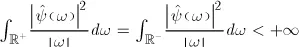
Let ψ be a sufficiently regular and well localized function. This function ψ ∈. L1 ∩ L2 will be called a wavelet if it verifies the following admissibility condition in the frequency domain:
where
indicates the Fourier transform of
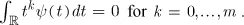
ψ. This condition involves, in particular, that the wavelet integrates to zero. This basic requirement is often reinforced by requiring that the wavelet has
m vanishing moments, i.e. verify
.
A sufficient admissibility condition that is much simpler to verify is, for a real wavelet ψ, provided by:
To consolidate the ideas let us say that during a certain time a wavelet oscillates like a wave and is then localized due to a damping. The oscillation of a wavelet is measured by the number of vanishing moments and its localization is evaluated by the interval where it takes values significantly different from zero.
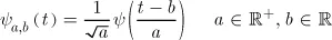
From this single function ψ using translation and dilation we build a family of functions that form the basic atoms:
For a function f of finite energy we define its continuous wavelet transform by the functionCf:
Calculating this function
Cf amounts to analyzing
f with the wavelet
ψ. The function
f is then described by its wavelet coefficients
Cf (
a,b), where a ∈
+ and
b ∈
. They measure the fluctuations of function
f at scale
a. The trend at scale
a containing slower evolutions is essentially eliminated in
Cf (
a,b). The analysis in wavelets makes a local analysis of
f possible, as well as the description of scale effects comparing the
Cf (
a,b) for various values of
a. Indeed, let us suppose that
ψ is zero outside of [−
M,+
M], so
ψa,b is...