Generalized, Linear, and Mixed Models

Charles E. McCulloch, Shayle R. Searle, John M. Neuhaus

• Publisher: Wiley-Interscience
• Year: 2011
• Print ISBN: 9780470073711
• eBook ISBN: 9781118209967
• Edition: 2
• Topic: Social Sciences
• Subtopic: Social Science Research & Methodology
• Index: Social Sciences

An accessible and self-contained introduction to statistical models-now in a modernized new edition Generalized, Linear, and Mixed Models, Second Edition provides an up-to-date treatment of the essential techniques for developing and applying a wide variety of statistical models. The book presents thorough and unified coverage of the theory behind generalized, linear, and mixed models and highlights their similarities and differences in various construction, application, and computational aspects. A clear introduction to the basic ideas of fixed effects models, random effects models, and mixed models is maintained throughout, and each chapter illustrates how these models are applicable in a wide array of contexts. In addition, a discussion of general methods for the analysis of such models is presented with an emphasis on the method of maximum likelihood for the estimation of parameters. The authors also provide comprehensive coverage of the latest statistical models for correlated, non-normally distributed data. Thoroughly updated to reflect the latest developments in the field, the Second Edition features:

• A new chapter that covers omitted covariates, incorrect random effects distribution, correlation of covariates and random effects, and robust variance estimation
• A new chapter that treats shared random effects models, latent class models, and properties of models
• A revised chapter on longitudinal data, which now includes a discussion of generalized linear models, modern advances in longitudinal data analysis, and the use between and within covariate decompositions
• Expanded coverage of marginal versus conditional models
• Numerous new and updated examples

With its accessible style and wealth of illustrative exercises, Generalized, Linear, and Mixed Models, Second Edition is an ideal book for courses on generalized linear and mixed models at the upper-undergraduate and beginning-graduate levels. It also serves as a valuable reference for applied statisticians, industrial practitioners, and researchers.

Chapter 1

INTRODUCTION

1.1 MODELS

a. Linear models (LM) and linear mixed models (LMM)

In almost all uses of statistics, major interest centers on averages and on variation about those averages. For more than sixty years this interest has frequently manifested itself in the widespread use of analysis of variance (ANOVA), as originally developed by R. A. Fisher. This involves expressing an observation as a sum of a mean plus differences between means, which, under certain circumstances, leads to methods for making inferences about means or about the nature of variability. The usually-quoted set of circumstances which permits this is that the expected value of each datum be taken as a linear combination of unknown parameters, considered as constants; and that the data be deemed to have come from a normal distribution. Thus the linear requirement is such that the expected value (i.e., mean), μ_ij, of a random observation y_ij can be, for example, of the form μ_ij= μ+ α_i+ β_j where μ, α_i and β_j are unknown constants — unknown, but which we want to estimate. And the normality requirement would be that y_ij is normally distributed with mean μ_ij. These requirements are the essence of what we call a linear model, or LM for short. By that we mean that the model is linear in the parameters, so “linearity” also includes being of the form

, for example, where the xs are known and there can be (and often are) more than two of them.

A variant of LMs is where parameters in an LM are treated not as constants but as (realizations of) random variables. To denote this different meaning we represent parameters treated as random by Roman rather than Greek letters. Thus if the as in the example were to be considered random, they would be denoted by as, so giving μ_ij= μ+ α_i+ β_j. With the βs remaining as constants, μ_ij is then a mixture of random and constant terms. Correspondingly, the model (which is still linear) is called a linear mixed model, or LMM. Until recently, most uses of such models have involved treating random α_is as having zero mean, being homoscedastic (i.e., having equal variance) with variance

and being uncorrelated. Additionally, normality of the α_is is usually also invoked.

There are many books dealing at length with LMs and LMMs. We name but a few: Graybill (1976), Seber (1977), Arnold (1981), Hocking (1985), Searle (1997), and Searle et al. (1992).

b. Generalized models (GLMs and GLMMs)

The last twenty-five years or so have seen LMs and LMMs extended to generalized linear models (GLMs) and to generalized linear mixed models (GLMMs). The essence of this generalization is two-fold: one, that data are not necessarily assumed to be normally distributed; and two, that the mean is not necessarily taken as a linear combination of parameters but that some function of the mean is. For example, count data may follow a Poisson distribution, with mean λ, say; and log λ will be taken as a linear combination of parameters. If all the parameters are considered as fixed constants the model is a GLM; if some are treated as random it is a GLMM.

The methodology for applying a GLM or a GLMM to data can be quite different from that for an LM or LMM. Nevertheless, some of the latter is indeed a basis for contributing to analysis procedures for GLMs and GLMMs, and to that extent this book does describe some of the procedures for LMs (Chapter 4) and LMMs (Chapter 6); Chapters 5 and 7 then deal, respectively, with GLMs and GLMMs. Chapters 2 and 3 provide details for the basic modeling of the one-way classification and of regression, prior to the general cases treated later.

1.2 FACTORS, LEVELS, CELLS, EFFECTS AND DATA

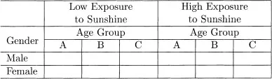
We are often interested in attributing the variability that is evident in data to the various categories, or classifications, of the data. For example, in a study of basal cell epithelioma sites (akin to Abu-Libdeh et al., 1990), patients might be classified by gender, age-group and extent of exposure to sunshine. The various groups of data could be summarized in a table such as Table 1.1.

The three classifications, gender, age, and exposure to sunshine, which identify the source of each datum are called factors. The individual classes of a classification are the levels of a factor (e.g., male and female are the two levels of the factor “gender”). The subset of data occurring at the “intersection” of one level of every factor being considered is said to be in a cell of the data. Thus with the three factors, gender (2 levels), age (3 levels) and sunshine (2 levels), there are 2 × 3 × 2 = 12 cells.

Table 1.1: A Format for Summarizing Data

Table 1.2: Summarizing Exam Grades

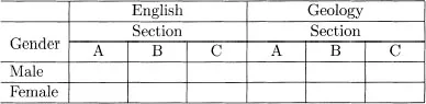
Suppose that we have student exam grades from each of three sections in English and Geology courses. The data could be summarized as in Table 1.2, similar to Table 1.1. Although the layout of Table 1.2 has the same appearance as Table 1.1, sections in Table 1.2 are very different from the age groups of Table 1.1. In Table 1.2 section A of English has no connection to (and will have different students from) section A of Geology; in the same way neither are sections B (or C) the same in the two subjects. Thus the section factor is nested within the subject factor. In contrast, in Table 1.1 the three age groups are the same for both low and high exposures to sunshine. The age and sunshine factors are said to be crossed.

In classifying data in terms of factors and their levels, the feature of interest is the extent to which different levels of a factor affect the variable of interest. We refer to this as the effect of a level of a factor on that variable. The effects of a factor are always one or other of two kinds, as introduced in Section 1.1 in terms of parameters. First is the case of parameters being considered as fixed constants or, as we henceforth call them, fixed effects. These are the effects attributable to a finite set of levels of a factor that occur in the data and which are there because we are interested in them. In Table 1.1 the effects for all three factors are fixed effects.

The second case corresponds to what we earlier described as parameters being considered random, now to be called random effects. These are attributable to a (usually) infinite set of levels of a factor, of which only a random sample are deemed to occur in the data. For example, four loaves of bread are taken from each of six batches of bread baked at three different temperatures. Since there is definite interest in the particular baking temperatures used, the statistical concern is to estimate those temperature effects; they are fixed effects. No assumption is made that the temperature effects are random. Indeed, even if the temperatures themselves were chosen at random, it would not be sensible to assume that the temperature effects were random. This is because temperature is defined on a continuum and, for example, the effect of a temperature of 450.11° is almost always likely to be a very similar to the effect of a 450.12° temperature. This nullifies the idea of temperature effects being random.

In contrast, batches are not defined on a continuum. They are real objects, just as are people, or cows, or clinics and so, depending on the circumstance, it can be perfectly reasonable to think of their effects as being random. Moreover, we can do this even if the objects themselves have not been chosen as a random sample — which, indeed, they seldom are. ...

Table of contents

• Cover
• Series
• Title
• Copyright
• Preface
• Preface First Edition
• CHAPTER 1: INTRODUCTION
• CHAPTER 2: ONE-WAY CLASSIFICATIONS
• CHAPTER 3: SINGLE-PREDICTOR REGRESSION
• CHAPTER 4: LINEAR MODELS (LMs)
• CHAPTER 5: GENERALIZED LINEAR MODELS (GLMs)
• CHAPTER 6: LINEAR MIXED MODELS (LMMs)
• CHAPTER 7: GENERALIZED LINEAR MIXED MODELS (GLMMs)
• CHAPTER 8: MODELS FOR LONGITUDINAL DATA
• CHAPTER 9: MARGINAL MODELS
• CHAPTER 10: MULTIVARIATE MODELS
• CHAPTER 11: NONLINEAR MODELS
• CHAPTER 12: DEPARTURES FROM ASSUMPTIONS
• CHAPTER 13: PREDICTION
• CHAPTER 14: COMPUTING
• Appendix 1
• Appendix 2
• References
• Index