Numerical Methods in Finance and Economics

A MATLAB-Based Introduction

Paolo Brandimarte

• Publisher: Wiley-Interscience
• Year: 2013
• ISBN:
  9781118625576
• Edition: 2
• Topic: Mathematics
• Subtopic: Probability & Statistics
• Index: Mathematics

A state-of-the-art introduction to the powerful mathematical and statistical tools used in the field of finance The use of mathematical models and numerical techniques is a practice employed by a growing number of applied mathematicians working on applications in finance. Reflecting this development, Numerical Methods in Finance and Economics: A MATLAB?-Based Introduction, Second Edition bridges the gap between financial theory and computational practice while showing readers how to utilize MATLAB?--the powerful numerical computing environment--for financial applications. The author provides an essential foundation in finance and numerical analysis in addition to background material for students from both engineering and economics perspectives. A wide range of topics is covered, including standard numerical analysis methods, Monte Carlo methods to simulate systems affected by significant uncertainty, and optimization methods to find an optimal set of decisions. Among this book's most outstanding features is the integration of MATLAB?, which helps students and practitioners solve relevant problems in finance, such as portfolio management and derivatives pricing. This tutorial is useful in connecting theory with practice in the application of classical numerical methods and advanced methods, while illustrating underlying algorithmic concepts in concrete terms. Newly featured in the Second Edition:
* In-depth treatment of Monte Carlo methods with due attention paid to variance reduction strategies
* New appendix on AMPL in order to better illustrate the optimization models in Chapters 11 and 12
* New chapter on binomial and trinomial lattices
* Additional treatment of partial differential equations with two space dimensions
* Expanded treatment within the chapter on financial theory to provide a more thorough background for engineers not familiar with finance
* New coverage of advanced optimization methods and applications later in the text
Numerical Methods in Finance and Economics: A MATLAB?-Based Introduction, Second Edition presents basic treatments and more specialized literature, and it also uses algebraic languages, such as AMPL, to connect the pencil-and-paper statement of an optimization model with its solution by a software library. Offering computational practice in both financial engineering and economics fields, this book equips practitioners with the necessary techniques to measure and manage risk.

Part I

Background

1

Motivation

Common wisdom would probably associate the ideas of numerical methods and number crunching to problems in science and engineering, rather than finance. This intuitive view is contradicted by the relatively large number of books and scientific journals devoted to computational finance; even more so, by the fact, that these methods are not confined to academia, but are actually used in real life. As a result, there has been a steady increase in the number of academic programs devoted to quantitative finance, both at Master’s and Ph.D. level, and they usually include a course on numerical methods. Furthermore, many people with a quantitative or numerical analysis background have started working in finance, including engineers, mathematicians, and physicists.

Indeed, as the term financial engineering may suggest, computational finance is a field where different cultures meet. Hence, a wide array of students and practitioners, with diverse background, will hopefully be interested in a book on numerical methods for finance. On the one hand, this is good news for the author. On the other one, the first difficult task is to get everyone on common ground as far as financial theory and the basics of numerical analysis are concerned; if treatment is too brief, there is a significant risk of losing a considerable subset of readers along the way; if it is too detailed, another subset will be considerably bored. The aim of the first three chapters is to “synchronize” readers with a background in Finance and readers with a scientific background, including students in Engineering, Mathematics, and Physics. In chapter 2, we will give the second subset of readers an overview of concepts in finance, with an emphasis on asset pricing and portfolio management. The first subset of readers will find a reasonably self-contained treatment on classical topics of numerical analysis in chapter 3.

In this introductory chapter we want to give a preview of the problems we will deal with, along with some motivation. The reader who is unfamiliar with some topics just outlined here should not be worried, as they are not taken for granted and will be treated thoroughly in the next chapters. We want to make three points:

1. In financial engineering we need numerical methods (section 1.1).

2. We need sophisticated and user-friendly numerical computing environments, such as MATLAB¹ (section 1.2), even if this does not prevent at all the use of (relatively) low-level languages such as Fortran or C++ or spreadsheets such as Microsoft Excel.

3. Whatever software tool we select, we need a reasonably strong theoretical background, as we must often select among competing methods and many things may go wrong with them (section 1.3).

1.1 NEED FOR NUMERICAL METHODS

Probably, the best-known result in financial engineering is the Black–Scholes formula to price options on stocks.² Options are a class of derivatives, i.e., financial assets whose value depends on another asset, called the underlying. The underlying can also be a non-financial asset, such as a commodity, or an arbitrary quantity representing a risk factor to someone, such as weather, so that setting up a market to transfer risks makes sense. Options are contracts with very specific rules for issuing, trading, and accounting. For instance, a European-style call option on a stock gives the holder the right, but not the obligation, of buying a given stock at a given time (maturity, denoted by T), for a prespecified price (the strike price, denoted by K). Similarly, a put option gives the right to sell the underlying asset at a predetermined strike price. In European-style derivatives, the right specified in the contract can only be exercised at maturity T; in American-style derivatives, one can exercise her right at any time before T, which in this case plays the role of the expiration date of the option.

In the case of a European-style call option, if the asset price at maturity is S(T), then the payoff is max{S(T) – K, 0}. The rationale here is that, under idealized assumptions on financial markets, the option holder could purchase the underlying asset at the prevailing price S(T) and immediately sell it at price K. Clearly, the option holder will do so only if this results in a positive profit. Actually, market imperfections, such as transaction costs or bid–ask spreads, prevent such an idealized trade: even if S(T) is the last quoted price, there is no guarantee that the option holder can actually buy the stock at that price. In the book we will neglect such issues, which are related to the micro-structure of financial markets.

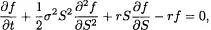
If we are at a time instant t < T, we would like to assign a value, or a fair price, to the option. However, what we know is only the current price S(t) of the underlying asset, whereas its price S(T) at maturity is not known. If we build some mathematical model for the dynamics of the price S(t) as a function of time, we may regard S(T) as a random variable; hence, the payoff is random as well, and there seems to be no trivial way to price this contract. Let f (S(t), t) be the price of the option at time t if the current price of the underlying asset is S(t); to ease the notation burden we will usually write it as f (S, t). It can be shown that, under suitable assumptions, the value of the contract really depends only on t and S, and it satisfies the following partial differential equation (PDE):

(1.1)

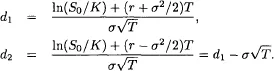
where r is the risk-free interest rate, i.e., the rate of interest one can earn by investing her money in a safe account, and σ is a parameter related to the volatility of the price of the underlying asset, which is a risky asset. Typically, we are interested in the current value f (So,0), where So = S(0). Equation (1.1), with the addition of suitable boundary conditions linked to the type of option, may be solved analytically in some cases. For instance, if we denote the cumulative distribution function³ for the standard normal distribution by N(z) = P{Z ≤ z}, where Z is a standard normal variable, the price C₀ for a European call option at time t = 0 is

(1.2)

where

This formula is easy to evaluate, but in general we are not so lucky. The complexity of the PDE or of some additional conditions, which we must impose to fully characterize a specific option, may require numerical methods. We will cover relatively simple numerical methods for solving PDEs, based on finite differences, in chapter 5, and applications to option pricing will be illustrated in chapter 9. Using finite differences, in turn, may call for the repeated solution of systems of linear equations, which is among the topics of chapter 3 on numerical analysis.

Apart from the obvious computational advantage, analytical formulas are of great importance in gaining insights into how different factors affect option prices. They also allow quick calculation of price sensitivities with respect to such factors, which are relevant for risk management. In the book, we will use analytical formulas quite often in order to validate numerical methods, by comparing the numerical result with the theoretically correct one. This is of no practical value by itself, but it is very instructive. Finally, we will also see that when a complex option cannot be priced analytically, knowing an analytical pricing formula for a related simpler option can be of great value. In option pricing by Monte Carlo simulation (see below), analytical pricing formulas may yield control variates useful to reduce variance in the estimate of price.

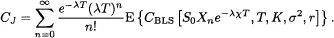
Nevertheless, we should note that the distinction between numerical and analytical methods is sometimes a bit blurred. It may happen that analytical formulas are quite complicated. As an example, let us consider the following formula, which we give without much explanation⁴:

This is a formula for the price of a European-style call option when price jumps are included in the model. The Black–Scholes model assumes continuous paths for prices, and this formula by Robert Merton generalizes to a model in which jumps occur according to a compound Poisson process. Here C_BLS(S, T, K, σ², r) is the standard Black–Scholes formula with the usual input arguments; λ is related to the rate of j...