![]()
CHAPTER 1
GENERALITIES
1.1 WHY ROBUST PROCEDURES?
Statistical inferences are based only in part upon the observations. An equally important base is formed by prior assumptions about the underlying situation. Even in the simplest cases, there are explicit or implicit assumptions about randomness and independence, about distributional models, perhaps prior distributions for some unknown parameters, and so on.
These assumptions are not supposed to be exactly true—they are mathematically convenient rationalizations of an often fuzzy knowledge or belief. As in every other branch of applied mathematics, such rationalizations or simplifications are vital, and one justifies their use by appealing to a vague continuity or stability principle: a minor error in the mathematical model should cause only a small error in the final conclusions.
Unfortunately, this does not always hold. Since the middle of the 20th century, one has become increasingly aware that some of the most common statistical procedures (in particular, those optimized for an underlying normal distribution) are excessively sensitive to seemingly minor deviations from the assumptions, and a plethora of alternative “robust” procedures have been proposed.
The word “robust” is loaded with many—sometimes inconsistent—connotations. We use it in a relatively narrow sense: for our purposes, robustness signifies insensitivity to small deviations from the assumptions.
Primarily, we are concerned with distributional robustness : the shape of the true underlying distribution deviates slightly from the assumed model (usually the Gaussian law). This is both the most important case and the best understood one. Much less is known about what happens when the other standard assumptions of statistics are not quite satisfied and about the appropriate safeguards in these other cases.
The following example, due to Tukey (1960), shows the dramatic lack of distributional robustness of some of the classical procedures.
Assume that we have a large, randomly mixed batch of
n “good” and “bad” observations
xi of the same quantity
μ. Each single observation with probability 1 –
ε is a “good” one, with probability
ε a “bad” one, where
ε is a small number. In the former case
xi is
(
μ, σ2), in the latter
(
μ, 9
σ2). In other words all observations are normally distributed with the same mean, but the errors of some are increased by a factor of 3.
Equivalently, we could say that the xi are independent, identically distributed with the common underlying distribution
where
is the standard normal cumulative.
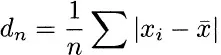
Two time-honored measures of scatter are the mean absolute deviation
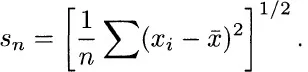
and the root mean square deviation
There was a dispute between Eddington (1914, p. 147) and Fisher (1920, footnote on p. 762) about the relative merits of dn and sn. Eddington had advocated the use of the former: “This is contrary to the advice of most textbooks; but it can be shown to be true.” Fisher seemingly settled the matter by pointing out that for identically distributed normal observations sn is about 12% more efficient than dn.
Of course, the two statistics measure different characteristics of the error distribution. For instance, if the errors are exactly normal,
sn converges to
σ, while
dn converges to
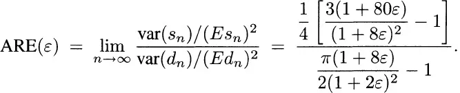
So we must be precise about how their performances are to be compared; we use the asymptotic relative efficiency (ARE) of
dn relative to
sn, defined as follows:
The results are summarized in Exhibit 1.1.
Exhibit 1.1 Asymptotic efficiency of mean absolute deviation relative to root mean square deviation. From Huber (1977b), with permission of the publisher.
| 0 | 0.876 |
| 0.001 | 0.948 |
| 0.002 | 1.016 |
| 0.005 | 1.198 |
| 0.01 | 1.439 |
| 0.02 | 1.752 |
| 0.05 | 2.035 |
| 0.10 | 1.903 |
| 0.15 | 1.689 |
| 0.25 | 1.371 |
| 0.5 | 1.017 |
| 1.0 | 0.876 |
The result is disquieting: just 2 bad observations in 1000 suffice to offset the 12% advantage of the mean square error, and ARE(ε) reaches a maximum value greater than 2 at about ε = 0.05. This is particularly unfortunate since in the physical sciences typical “good data” samples appear to be well modeled by an error law of the form (1.1) with ε in the range between 0.01 and 0.1. (This does not imply that these samples contain between 1% and 10% gross errors, although this is very often true; the above law (1.1) may just be a convenient description of a slightly longer-tailed than normal distribution.) Thus it becomes painfully clear that the naturally occurring deviations from the idealized model are large enough to render meaningless the traditional asymptotic optimal...