This is the first book devoted entirely to Particle Swarm Optimization (PSO), which is a non-specific algorithm, similar to evolutionary algorithms, such as taboo search and ant colonies.
Since its original development in 1995, PSO has mainly been applied to continuous-discrete heterogeneous strongly non-linear numerical optimization and it is thus used almost everywhere in the world. Its convergence rate also makes it a preferred tool in dynamic optimization.
As regards optimization, certain problems are regarded as more difficult than others. This is the case, inter alia, for combinatorial problems. But what does that mean? Why should a combinatorial problem necessarily be more difficult than a problem in continuous variables and, if this is the case, to what extent is it so? Moreover, the concept of difficulty is very often more or less implicitly related to the degree of sophistication of the algorithms in a particular research field: if one cannot solve a particular problem, or it takes a considerable time to do so, therefore it is difficult.
Later, we will compare various algorithms on various problems, and we will therefore need a rigorous definition. To that end, let us consider the algorithm for purely random research. It is often used as a reference, because even a slightly intelligent algorithm must be able to do better (even if it is very easy to make worse, for example an algorithm being always blocked in a local minimum). Since the measurement of related difficulty is very seldom clarified (see however [BAR 05]), we will do it here quickly.
The selected definition is as follows: the difficulty of an optimization problem in a given search space is the probability of not finding a solution by choosing a position at random according to a uniform distribution. It is thus the probability of failure at the first attempt.
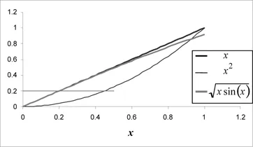
Consider the following examples. Take the function f defined in [0 1] by f(x) = x. The problem is “to find the minimum of this function nearest within s”. It is easy to calculate (assuming that
is less than 1) that the difficulty of this problem, following the definition above, is given by the quantity (1 – ε). As we can see in Figure 1.1, it is simply the ratio of two measurements: the total number of acceptable solutions and the total number of possible positions (in fact, the definition of a probability). From this point of view, the minimization of x2 is twice as easy as that of x.
Figure 1.1.Assessing the difficulty. The intrinsic difficulty of a problem of the minimization of a function (in this case, the search for an item x for which f(x) is less than 0.2) has nothing to do with the apparent complication of the formula of the function. On the search space [0 1], it is the function x2 that is by far the easiest, whereas there is little to choose between the two others, function x being very slightly more difficult
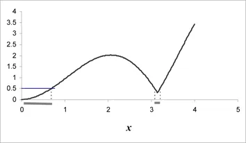
It should be noted that this assessment of difficulty can depend on the presence of local minima. For example, Figure 1.2 represents part of the graph of a variant of the so-called “Alpine” function, f (x) = |xsin(x) + 0.1x|. For
= 0.5 the field of the acceptable solutions is not connected. Of course, a part contains the position of the global minimum (0), but another part surrounds that of a local minimum whose value is less than ε. In other words, if the function presents local minima, and particularly if their values are close to that of the global minimum, one is quite able to obtain a satisfactory mathematical solution, but whose position is nevertheless very far from the hoped for solution.
By reducing the tolerance level (the acceptable error), one can certainly end up selecting only solutions actually located around the global minimum, but this procedure obviously increases the practical difficulty of the problem. Conversely, therefore, one tries to reduce the search space. But this requires some knowledge of the position of the solution sought and, moreover, it sometimes makes it necessary to define a search space that is more complicated than a simple Cartesian product of intervals; for example, a polyhedron, which may even be non-convex. However, we will see that this second item can be discussed in PSO by an option that allows an imperative constraint of the type g(position) < 0 to be taken into account.
Figure 1.2.A non-connected set of solutions. If the tolerance level is too high (here 0.5), some solutions can be found around a local minimum. Two different methods of avoiding this problem when searching for a global minimum are to reduce the tolerance level (which increases the practical difficulty of research) or to reduce the search space (which decreases the difficulty). But this second method requires that we have at least a vague idea of the position of the sought minimum
1.2. Estimation and practical measurement
When high precision is required, the probability of failure is very high and to take it directly as a measure of difficulty is not very practical. Thus we will use instead a logarithmic measurement given by the following formula:
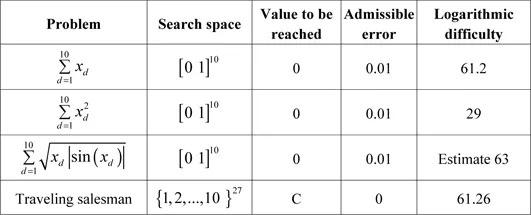
In this way one obtains more easily comparable numbers. Table 1.1 presents the results for four small problems. In each case, it is a question of reaching a minimal value. For the first three, the functions are continuous and one must accept a certain margin of error because that is what makes it possible to calculate the probability of success. The last problem is a classic “traveling salesman problem” with 27 cities, for which only one solution is supposed to exist. Here, the precision required is absolute: one wants to obtain this solution exactly.
Table 1.1.Difficulty of four problems compared. When the probabilities of success are very low, it is easier to compare their logarithms. The ways of calculating the difficulty are given at the end of the chapter. For the third function, it is only a rather pessimistic statistical estimate (in reality, one should be able to find a value less than the difficulty of the first function). For the traveling salesman problem (search for a Hamiltonian cycle of minimal length), it was supposed that there was only one solution, of value C; it must be reached exactly, without any margin of error
We see, for example, that the first and last problems are of the same level of intrinsic difficulty. It is therefore not absurd to imagine that the same algorithm, particularly if it uses randomness advisedly, can solve one as well as the other. Moreover, and we will return to this, the distinction between discrete/combinatorial problems and continuous problems is rather arbitrary for at least two reasons:
– a continuous problem becomes necessarily discrete, since it is treated on a numerical computer, hence with limited precision;
– a discrete problem can be replaced by an equivalent continuous problem under constraints, by interpolating the function defining it on the search space.
1.3. For “amatheurs”: some estimates of difficulty
The probability of success can be estimated in various ways, according to the form of the function:
– direct calculation by integration in the simple cases;
– calculation on a finite expansion, either of the function itse...
Table of contents
Cover
Title Page
Copyright
Foreword
Introduction
Part I: Particle Swarm Optimization
Part II: Outlines
Further Information
Bibliography
Index
Frequently asked questions
Yes, you can cancel anytime from the Subscription tab in your account settings on the Perlego website. Your subscription will stay active until the end of your current billing period. Learn how to cancel your subscription
No, books cannot be downloaded as external files, such as PDFs, for use outside of Perlego. However, you can download books within the Perlego app for offline reading on mobile or tablet. Learn how to download books offline
Perlego offers two plans: Essential and Complete
Essential is ideal for learners and professionals who enjoy exploring a wide range of subjects. Access the Essential Library with 800,000+ trusted titles and best-sellers across business, personal growth, and the humanities. Includes unlimited reading time and Standard Read Aloud voice.
Complete: Perfect for advanced learners and researchers needing full, unrestricted access. Unlock 1.4M+ books across hundreds of subjects, including academic and specialized titles. The Complete Plan also includes advanced features like Premium Read Aloud and Research Assistant.
Both plans are available with monthly, semester, or annual billing cycles.
We are an online textbook subscription service, where you can get access to an entire online library for less than the price of a single book per month. With over 1 million books across 990+ topics, we’ve got you covered! Learn about our mission
Look out for the read-aloud symbol on your next book to see if you can listen to it. The read-aloud tool reads text aloud for you, highlighting the text as it is being read. You can pause it, speed it up and slow it down. Learn more about Read Aloud
Yes! You can use the Perlego app on both iOS and Android devices to read anytime, anywhere — even offline. Perfect for commutes or when you’re on the go. Please note we cannot support devices running on iOS 13 and Android 7 or earlier. Learn more about using the app
Yes, you can access Particle Swarm Optimization by Maurice Clerc in PDF and/or ePUB format, as well as other popular books in Computer Science & Artificial Intelligence (AI) & Semantics. We have over one million books available in our catalogue for you to explore.