Pairs Trading

Quantitative Methods and Analysis

Ganapathy Vidyamurthy

• Publisher: Wiley
• Year: 2011
• ISBN:
  9781118045701
• Edition: 1
• Topic: Betriebswirtschaft
• Subtopic: Finanzwesen

The first in-depth analysis of pairs trading
Pairs trading is a market-neutral strategy in its most simple form. The strategy involves being long (or bullish) one asset and short (or bearish) another. If properly performed, the investor will gain if the market rises or falls. Pairs Trading reveals the secrets of this rigorous quantitative analysis program to provide individuals and investment houses with the tools they need to successfully implement and profit from this proven trading methodology. Pairs Trading contains specific and tested formulas for identifying and investing in pairs, and answers important questions such as what ratio should be used to construct the pairs properly.
Ganapathy Vidyamurthy (Stamford, CT) is currently a quantitative software analyst and developer at a major New York City hedge fund.

PART One

Background Material

CHAPTER 1

Introduction

We start at the very beginning (a very good place to start). We begin with the CAPM model.

THE CAPM MODEL

CAPM is an acronym for the Capital Asset Pricing Model. It was originally proposed by William T. Sharpe. The impact that the model has made in the area of finance is readily evident in the prevalent use of the word beta. In contemporary finance vernacular, beta is not just a nondescript Greek letter, but its use carries with it all the import and implications of its CAPM definition.

Along with the idea of beta, CAPM also served to formalize the notion of a market portfolio. A market portfolio in CAPM terms is a portfolio of assets that acts as a proxy for the market. Although practical versions of market portfolios in the form of market averages were already prevalent at the time the theory was proposed, CAPM definitely served to underscore the significance of these market averages.

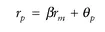
Armed with the twin ideas of market portfolio and beta, CAPM attempts to explain asset returns as an aggregate sum of component returns. In other words, the return on an asset in the CAPM framework can be separated into two components. One is the market or systematic component, and the other is the residual or nonsystematic component. More precisely, if r_p is the return on the asset, r_m is the return on the market portfolio, and the beta of the asset is denoted as β, the formula showing the relationship that achieves the separation of the returns is given as

(1.1)

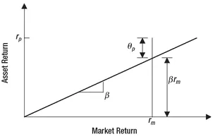
Equation 1.1 is also often referred to as the security market line (SML). Note that in the formula, βr_m is the market or systematic component of the return. β serves as a leverage number of the asset return over the market return. For instance, if the beta of the asset happens to be 3.0 and the market moves 1 percent, the systematic component of the asset return is now 3.0 percent. This idea is readily apparent when the SML is viewed in geometrical terms in Figure 1.1. It may also be deduced from the figure that β is indeed the slope of the SML.

θ_p in the CAPM equation is the residual component or residual return on the portfolio. It is the portion of the asset return that is not explainable by the market return. The consensus expectation on the residual component is assumed to be zero.

Having established the separation of asset returns into two components, CAPM then proceeds to elaborate on a key assumption made with respect to the relationship between them. The assertion of the model is that the market component and residual component are uncorrelated. Now, many a scholarly discussion on the import of these assumptions has been conducted and a lot of ink used up on the significance of the CAPM model since its introduction. Summaries of those discussions may be found in the references provided at the end of the chapter. However, for our purposes, the preceding introduction explaining the notion of beta and its role in the determination of asset returns will suffice.

FIGURE 1.1 The Security Market Line.

Given that knowledge of the beta of an asset is greatly valuable in the CAPM context, let us discuss briefly how we can go about estimating its value. Notice that beta is actually the slope of the SML. Therefore, beta may be estimated as the slope of the regression line between market returns and the asset returns. Applying the standard regression formula for the estimation of the slope we have

(1.2)

that is, beta is the covariance between the asset and market returns divided by the variance of the market returns.

To see the typical range of values that the beta of an asset is likely to assume in practice, we remind ourselves of an oft-quoted adage about the markets, “A rising tide raises all boats.” The statement indicates that when the market goes up, we can typically expect the price of all securities to go up with it. Thus, a positive return for the market usually implies a positive return for the asset, that is, the sum of the market component and the residual component is positive. If the residual component of the asset return is small, as we expect it to be, then the positive return in the asset is explained almost completely by its market component. Therefore, a positive return in the market portfolio and the asset implies a positive market component of the return and, by implication, a positive value for beta. Therefore, we can expect all assets to typically have positive values for their betas.

MARKET NEUTRAL STRATEGY

Having discussed CAPM, we now have the required machinery to define market neutral strategies: They are strategies that are neutral to market returns, that is, the return from the strategy is uncorrelated with the market return. Regardless of whether the market goes up or down, in good times and bad the market neutral strategy performs in a steady manner, and results are typically achieved with a lower volatility. This desired outcome is achieved by trading market neutral portfolios. Let us therefore define what we mean by a market neutral portfolio.

In the CAPM context, market neutral portfolios may be defined as portfolios whose beta is zero. To examine the implications, let us apply a beta value of zero to the equation for the SML. It is easy to see that the return on the portfolio ceases to have a market component and is completely determined by θ_p, the residual component. The residual component by the CAPM assumption happens to be uncorrelated with market returns, and the portfolio return is therefore neutral to the market. Thus, a zero beta portfolio qualifies as a market neutral portfolio.

In working with market neutral portfolios, the trader can now focus on forecasting and trading the residual returns. Since the consensus expectation or mean on the residual return is zero, it is reasonable to expect a strong mean-reverting behavior (value oscillates back and forth about the mean value) of the residual time series.¹ This mean-reverting behavior can then be exploited in the process of return prediction, leading to trading signals that constitute the trading strategy.

Let us now examine how we can construct market neutral portfolios and what we should expect by way of the composition of such portfolios. Consider a portfolio that is composed of strictly long positions in assets. We expect that beta of the assets to be positive. Then positive returns in the market result in a positive return for the assets and thereby a positive return for the portfolio. This would, of course, imply a positive beta for the portfolio. By a similar argument it is easy to see that a portfolio composed of strictly short positions is likely to have a negative beta. So, how do we construct a zero beta portfolio, using securities with positive betas? This would not be possible without holding both long and short positions on different assets in the portfolio. We there...