Spatial Statistics and Spatio-Temporal Data

Covariance Functions and Directional Properties

Michael Sherman

• Publisher: Wiley
• Year: 2011
• Print ISBN: 9780470699584
• eBook ISBN: 9780470974926
• Edition: 1
• Topic: Mathematics
• Subtopic: Probability & Statistics
• Index: Mathematics

In the spatial or spatio-temporal context, specifying the correct covariance function is fundamental to obtain efficient predictions, and to understand the underlying physical process of interest. This book focuses on covariance and variogram functions, their role in prediction, and appropriate choice of these functions in applications. Both recent and more established methods are illustrated to assess many common assumptions on these functions, such as, isotropy, separability, symmetry, and intrinsic correlation.

After an extensive introduction to spatial methodology, the book details the effects of common covariance assumptions and addresses methods to assess the appropriateness of such assumptions for various data structures.

Key features:

• An extensive introduction to spatial methodology including a survey of spatial covariance functions and their use in spatial prediction (kriging) is given.
• Explores methodology for assessing the appropriateness of assumptions on covariance functions in the spatial, spatio-temporal, multivariate spatial, and point pattern settings.
• Provides illustrations of all methods based on data and simulation experiments to demonstrate all methodology and guide to proper usage of all methods.
• Presents a brief survey of spatial and spatio-temporal models, highlighting the Gaussian case and the binary data setting, along with the different methodologies for estimation and model fitting for these two data structures.
• Discusses models that allow for anisotropic and nonseparable behaviour in covariance functions in the spatial, spatio-temporal and multivariate settings.
• Gives an introduction to point pattern models, including testing for randomness, and fitting regular and clustered point patterns. The importance and assessment of isotropy of point patterns is detailed.

Statisticians, researchers, and data analysts working with spatial and space-time data will benefit from this book as well as will graduate students with a background in basic statistics following courses in engineering, quantitative ecology or atmospheric science.

1

Introduction

Spatial statistics, like all branches of statistics, is the process of learning from data. Many of the questions that arise in spatial analyses are common to all areas of statistics. Namely,

i. What are the phenomena under study.

ii. What are the relevant data and how should it be collected.

iii. How should we analyze the data after it is collected.

iv. How can we draw inferences from the data collected to the phenomena under study.

The way these questions are answered depends on the type of phenomena under study. In the spatial or spatio-temporal setting, these issues are typically addressed in certain ways. We illustrate this from the following study of phosphorus measurements in shrimp ponds.

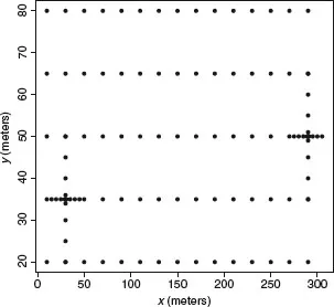
Figure 1.1 gives the locations of phosphorus measurements in a 300m × 100m pond in a Texas shrimp farm.

i. The phenomena under study are:

a. Are the observed measurements sufficient to measure total phosphorus in the pond? What can be gained in precision by further sampling?

b. What are the levels of phosphorus at unsampled locations in the pond, and how can we predict them?

c. How does the phosphorus level at one location relate to the amount at another location?

d. Does this relationship depend only on distance or also on direction?

Figure 1.1 Sampling locations of phosphorus measurements.

ii. The relevant data that are collected are as follows: a total of n = 103 samples were collected from the top 10 cm of the soil from each pond by a core sampler with a 2.5 cm diameter. We see 15 equidistant samples on the long edge (300 m), and 5 equidistant samples from the short edge (100 m). Additionally, 14 samples were taken from each of the shallow and deep edges of each pond. The 14 samples were distributed in a cross shape. Two of the sides of the cross consist of samples at distances of 1, 5, 10, and 15 m from the center while the remaining two have samples at 1, 5, and 10 m from the center.

iii. The analysis of the data shows that the 14 samples in each of the two cross patterns turn out to be very important for both the analysis, (iii), and inferences, (iv), drawn from these data. This will be discussed further in Section 3.5.

iv. Inferences show that the answer to (d) helps greatly in answering question (c), which in turn helps in answering question (b) in an informative and efficient manner. Further, the answers to (b), (c), and (d) determine how well we can answer question (a). Also, we will see that increased sampling will not give much better answers to (a); while addressing (c), it is found that phosphorus levels are related but only up to a distance of about 15–20 m. The exact meaning of ‘related,’ and how these conclusions are reached, are discussed in the next paragraph and in Chapter 2.

We consider all observed values to be the outcome of random variables observed at the given locations. Let {Z(s_i), i = 1,…, n} denote the random quantity Z of interest observed at locations

, where D is the domain where observations are taken, and d is the dimension of the domain. In the phosphorus study, Z(s_i) denotes the log(phosphorus) measurement at the ith sampling location, i = 1,…, 103. The dimension d is 2, and the domain D is the 300m × 100m pond. For usual spatial data, the dimension, d, is 2.

Sometimes the locations themselves will be considered random, but for now we consider them to be fixed by the experimenter (as they are, e.g., in the phosphorus study). A fundamental concept for addressing question (iii) in the first paragraph of the introduction is the covariance function.

For any two variables Z(s) and Z(t) with means μ(s) and μ(t), respectively, we define the covariance to be

The correlation function is then Cov[Z(s), Z(t)]/(σ_sσ_t), where σ_s and σ_t denote the standard deviations of the two variables. We see, for example, that if all random observations are independent, then the covariance and the correlation are identically zero, for all locations s and t, such that s ≠ t. In the special case where the mean and variances are constant, that is, μ(t) = μ and σ_s = σ for all locations s, we have

The covariance function, which is very important for prediction and inference, typically needs to be estimated. Without any replication this is usually not feasible. We next give a common assumption made in order to obtain replicates.

1.1 Stationarity

A standard method of obtaining replication is through the assumption of second-order stationarity (SOS). This assumption holds that:

i. E[Z(s)] = μ;

ii. Cov[Z(s), Z(t)] = Cov[Z(s + h), (t + h)] for all shifts h.

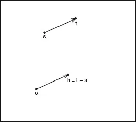
Figure 1.2 shows the locations for a particular shift vector h. In this case we can write

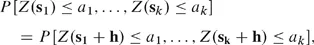
so that the covariance depends only on the spatial lag between the locations, t − s, and not on the two locations themselves. Second-order stationarity is often known as ‘weak stationarity.’ Strong (or strict) stationarity assumes that, for any collection of k variables, Z(s_i), i = 1,…, k, and constants a_i, i = 1,…, k, we have

for all shift vectors h.

Figure 1.2 A depiction of stationarity: two identical lag vectors.

This says that the entire joint distribution of k variables is invariant under shifts. Taking k = 1 and k = 2, and observing that covariances are determined by the joint distribution, it is seen that strong stationarity implies SOS. Generally, to answer the phenomenon of interest ...

Table of contents

• Cover
• Contents
• Half Title
• Series Page
• Book Title
• Copyright
• Preface
• Chapter 1: Introduction
• Chapter 2: Geostatistics
• Chapter 3: Variogram and covariance models and estimation
• Chapter 4: Spatial models and statistical inference
• Chapter 5: Isotropy
• Chapter 6: Space–time data
• Chapter 7: Spatial point patterns
• Chapter 8: Isotropy for spatial point patterns
• Chapter 9: Multivariate spatial and spatio-temporal models
• Chapter 10: Resampling for correlated observations
• Bibliography
• Index
• Series Title