Interest Rate Swaps and Their Derivatives

A Practitioner's Guide

Amir Sadr

• Publisher: Wiley
• Year: 2009
• Print ISBN: 9780470443941
• eBook ISBN: 9780470526118
• Edition: 1
• Topic: Business
• Subtopic: Finance
• Index: Business

An up-to-date look at the evolution of interest rate swaps and derivatives

Interest Rate Swaps and Derivatives bridges the gap between the theory of these instruments and their actual use in day-to-day life. This comprehensive guide covers the main "rates" products, including swaps, options (cap/floors, swaptions), CMS products, and Bermudan callables. It also covers the main valuation techniques for the exotics/structured-notes area, which remains one of the most challenging parts of the market.

• Provides a balance of relevant theory and real-world trading instruments for rate swaps and swap derivatives
• Uses simple settings and illustrations to reveal key results
• Written by an experienced trader who has worked with swaps, options, and exotics

With this book, author Amir Sadr shares his valuable insights with practitioners in the field of interest rate derivatives-from traders and marketers to those in operations.

PART One

Cash, Repo, and Swap Markets

CHAPTER 1

Bonds: It′s All About Discounting

Before we delve into all the good stuff (swaps and options), let us review some fixed income basics.

TIME VALUE OF MONEY: FUTURE VALUE, PRESENT VALUE

Following the classical fixed income gospels, we remember that the Future Value, FV, on a horizon date of an investment PV at an annual interest rate of r , compounded m times a year, for N whole compounding periods is

FV = PV(1+r/m)^N

For example, if m = 1, we have annual compounding FV = PV(1 + r )^N, and N is the number of years until the future horizon date. If m = 2, we have semiannual compounding (standard for U.S. Treasury securities) FV = PV(1 + r /2)^N, and N = 2T is the number of whole semiannual periods until the horizon date (T years from now).

The above formula can be easily generalized to incorporate horizon dates that are not a whole number of compounding periods away. We compute T as the number of years between the investment date and the horizon date, according to some day count basis, and come up with:

FV = PV(1 + r/m)^Tm

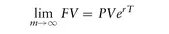
From college math courses, we recall that as you increase the compounding frequency, the above, in the limit, becomes

and r is then referred to as the continuous compounding rate.

An alternative to using compounded rates is to use simple or noncompounding interest rates:

FV = PV(1 + r T)

where T is the number of years (can be fractional) to the horizon date. Simple interest rates are usually used for Money Market instruments, that is, with maturity less than 1 year.

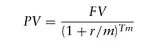
In order to compute how much money needs to be invested today at interest rate r , compounded m times a year, for T years to get FV at maturity, one simply inverts the above equation to come up with Present Value, PV:

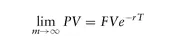
and in the limit:

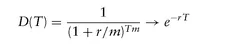
By setting FV to 1, PV becomes today′s price of unit currency to be received at time T, that is, present value of $1, and we will denote it by Discount Factor, D:

This would be price of a security that returns unit dollar at maturity (T years from now), that is, the price of a T-maturity zero-coupon bond, and provides an (implicit) yield r , compounded m times a year.

Note that while interest rates r can be quoted in different ways, the actual investment ( PV dollars in, FV dollars out) remains the same. In order to compare different investments, one would need to compare them using the same metric, that is, interest rates with the same quote convention. However, in order to value investments, all we need are discount factors.

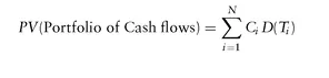
Discount factors are the fundamental building blocks for valuing fixed income securities. Given a series of known cash flows (C₁,...,C_N) to be received at various times (T₁ , . . . , T_N) in the future, if we know the discount factor D(T_i ) for each payment date T_i , then today′s value of this package is:

PRICE-YIELD FORMULA

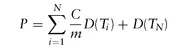
For example, today′s price P of a T-year bond paying an annualized coupon rate C, m times a year (so N = T × m payments left) is

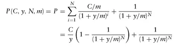
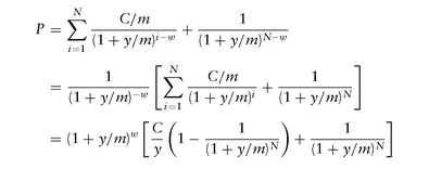
The standard bond pricing formula is based on Flat Yield assumption: it assumes that there is a single interest rate called Yield-to-Maturity (YTM) y applicable for all cash flows of the bond, regardless of how far the payment date is. With this assumption, D(T_i ) = 1/(1 + y/m)ⁱ , and we get the classical bond pricing formula:

The above formula is for when there are N = T × m whole future coupon periods left. For a bond in the middle of a coupon period, the discount factors get modified as D(T_i ) = 1/(1 + y/m)^{i -w} where w measures the accrued fraction (measured using some day-count convention: Act/Act, Act/365, . . .) of the current coupon period:

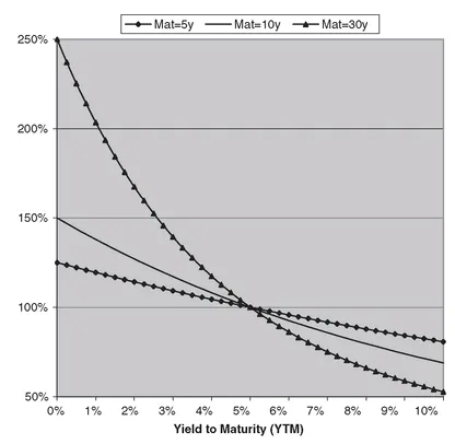
The above formula is the Dirty Price of a bond, that is, how much cash is needed in order to purchase this bond. One needs to always remember that dirty price of a bond is the discounted value of its remaining cash flows. The standard price/yield formulae simply express this via assuming a flat yield and expressing all discount factors as a function of this (hypothetical) yield y. Figure 1.1 shows the graph of Price as a function of YTM. As can be seen, when yield equals the coupon rate, the price of the bond is Par (100%). Also, longer-maturity bonds exhibit a higher curvature (convexity) in their price-yield relationship.

FIGURE 1.1 Price-Yield Graph for a 5% Semiannual Coupon Bond

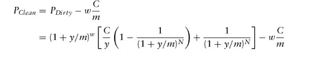
The graph of a dirty price of a bond versus time to maturity T is discontinuous, with drops (equal to paid coupon) on coupon payment dates. This makes sense, since the present value of remaining cash flows should drop when there is one less coupon. For bond traders focused on quoted price of a bond, this drop in price (while real in terms of PV of remaining cash flows) is artificial in terms of worthiness/value of a bond, and they prefer a smoother measure. By subtracting the accrued interest, wC/m from the dirty price, one arrives at the Clean/Quoted Price:

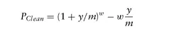
Note that when coupon rate equals yield, C = y, the term in the square brackets becomes 1, and the formula simplifies to

On coupon payment dates the accrued fraction w equals zero, and the price is par: P = 1 = 100%. In between coupon payment dates, even when C = y, the price is not exactly par. This is because the above formula is based on the Street Convention where fractional periods are adjusted using the formula suggested by compounded interest rates: 1/(1 + y/m)^-w = (1 + y/m)^w . 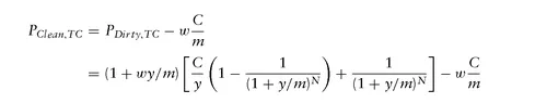If instead, we had used simple interest rates for first period, we would get the clean price using the Treasury Convention (TC):

and then the price of a bond when C = y would be par (100%) at all times.

Figure 1.2 shows the evolution of the clean and dirty prices for a 2y 5% semiannual coupon bond as we get closer to maturity while holding yields constant for 3 yield scenarios: y = 7.5% leading to a Premium bond (C < y), y = 2.5% leading to a Discount bond (C > y), and y = 5% leading to a par (C = y) bond. Notice the Pull-To-Par Effect for the bond regardless of the assumed yield scenario: A discount bond gets pulled up to par, while a premium bond gets pulled down to par.

In order to flesh out the calculation details, for the remainder of the chapter, we will focus on the 2y U.S. Treasury note issued on 1-Oct-2007, with CUSIP (Committee on Uniform Security Identification Procedures) number 912828HD5, shown in Table 1.1. From Announcement date till Auction date, these 2-year notes will be considered When-Issued (WI) and trade based on yield since the coupon rate is only known at Auction time. After the auction they start trading based on price, and become th...

Table of contents

• Title Page
• Copyright Page
• Preface
• About the Author
• List of Symbols and Abbreviations
• PART One - Cash, Repo, and Swap Markets
• PART Two - Interest-Rate Flow Options
• PART Three - Interest-Rate Exotics
• APPENDIX A - Taylor Series Expansion
• APPENDIX B - Mean-Reverting Processes
• APPENDIX C - Girsanov′s Theorem and Change of Numeraire
• Notes
• Index