The Handbook of Portfolio Mathematics

Formulas for Optimal Allocation & Leverage

Ralph Vince

• Publisher: Wiley
• Year: 2008
• Print ISBN: 9780471757689
• eBook ISBN: 9780470410509
• Edition: 1
• Topic: Business
• Subtopic: Investments & Securities
• Index: Business

The Handbook of Portfolio Mathematics

"For the serious investor, trader, or money manager, this book takes a rewarding look into modern portfolio theory. Vince introduces a leverage-space portfolio model, tweaks it for the drawdown probability, and delivers a superior model. He even provides equations to maximize returns for a chosen level of risk. So if you're serious about making money in today's markets, buy this book. Read it. Profit from it."
—Thomas N. Bulkowski, author, Encyclopedia of Chart Patterns

"This is an important book. Though traders routinely speak of their 'edge' in the marketplace and ways of handling 'risk, ' few can define and measure these accurately. In this book, Ralph Vince takes readers step by step through an understanding of the mathematical foundations of trading, significantly extending his earlier work and breaking important new ground. His lucid writing style and liberal use of practical examples make this book must reading."
—Brett N. Steenbarger, PhD, author, The Psychology of Trading and Enhancing Trader Performance

"Ralph Vince is one of the world's foremost authorities on quantitative portfolio analysis. In this masterly contribution, Ralph builds on his early pioneering findings to address the real-world concerns of money managers in the trenches-how to systematically maximize gains in relation to risk."
—Nelson Freeburg, Editor, Formula Research

"Gambling and investing may make strange bedfellows in the eyes of many, but not Ralph Vince, who once again demonstrates that an open mind is the investor's most valuable asset. What does bet sizing have to do with investing? The answer to that question and many more lie inside this iconoclastic work. Want to make the most of your investing skills Open this book."
—John Bollinger, CFA, CMT, www.BollingerBands.com

PART I

Theory

CHAPTER 1

The Random Process and Gambling Theory

We will start with the simple coin-toss case. When you toss a coin in the air there is no way to tell for certain whether it will land heads or tails. Yet over many tosses the outcome can be reasonably predicted.

This, then, is where we begin our discussion.

Certain axioms will be developed as we discuss the random process. The first of these is that the outcome of an individual event in a random process cannot be predicted. However, we can reduce the possible outcomes to a probability statement.

Pierre Simon Laplace (1749-1827) defined the probability of an event as the ratio of the number of ways in which the event can happen to the total possible number of events. Therefore, when a coin is tossed, the probability of getting tails is 1 (the number of tails on a coin) divided by 2 (the number of possible events), for a probability of .5. In our coin-toss example, we do not know whether the result will be heads or tails, but we do know that the probability that it will be heads is .5 and the probability it will be tails is .5. So, a probability statement is a number between 0 (there is no chance of the event in question occurring) and 1 (the occurrence of the event is certain).

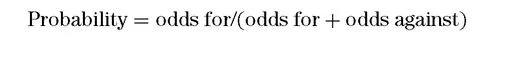
Often you will have to convert from a probability statement to odds and vice versa. The two are interchangeable, as the odds imply a probability, and a probability likewise implies the odds. These conversions are given now. The formula to convert to a probability statement, when you know the given odds is:

(1.01)

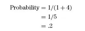
If the odds on a horse, for example, are 4 to 1 (4:1), then the probability of that horse winning, as implied by the odds, is:

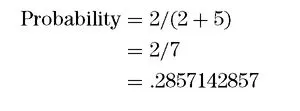
So a horse that is 4:1 can also be said to have a probability of winning of .2. What if the odds were 5 to 2 (5:2)? In such a case the probability is:

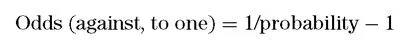
The formula to convert from probability to odds is:

(1.02)

So, for our coin-toss example, when there is a .5 probability of the coin’s coming up heads, the odds on its coming up heads are given as:

This formula always gives you the odds “to one.” In this example, we would say the odds on a coin’s coming up heads are 1 to 1.

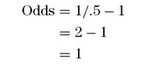
How about our previous example, where we converted from odds of 5:2 to a probability of .2857142857? Let’s work the probability statement back to the odds and see if it works out.

Here we can say that the odds in this case are 2.5 to 1, which is the same as saying that the odds are 5 to 2. So when someone speaks of odds, they are speaking of a probability statement as well.

Most people can’t handle the uncertainty of a probability statement; it just doesn’t sit well with them. We live in a world of exact sciences, and human beings have an innate tendency to believe they do not understand an event if it can only be reduced to a probability statement. The domain of physics seemed to be a solid one prior to the emergence of quantum physics. We had equations to account for most processes we had observed. These equations were real and provable. They repeated themselves over and over and the outcome could be exactly calculated before the event took place. With the emergence of quantum physics, suddenly a theretofore exact science could only reduce a physical phenomenon to a probability statement. Understandably, this disturbed many people.

I am not espousing the random walk concept of price action nor am I asking you to accept anything about the markets as random. Not yet, anyway. Like quantum physics, the idea that there is or is not randomness in the markets is an emotional one. At this stage, let us simply concentrate on the random process as it pertains to something we are certain is random, such as coin tossing or most casino gambling. In so doing, we can understand the process first, and later look at its applications. Whether the random process is applicable to other areas such as the markets is an issue that can be developed later.

Logically, the question must arise, “When does a random sequence begin and when does it end?” It really doesn’t end. The blackjack table continues running even after you leave it. As you move from table to table in a casino, the random process can be said to follow you around. If you take a day off from the tables, the random process may be interrupted, but it continues upon your return. So, when we speak of a random process of X events in length we are arbitrarily choosing some finite length in order to study the process.

INDEPENDENT VERSUS DEPENDENT TRIALS PROCESSES

We can subdivide the random process into two categories. First are those events for which the probability statement is constant from one event to the next. These we will call independent trials processes or sampling with replacement. A coin toss is an example of just such a process. Each toss has a 50/50 probability regardless of the outcome of the prior toss. Even if the last five flips of a coin were heads, the probability of this flip being heads is unaffected, and remains .5.

Naturally, the other type of random process is one where the outcome of prior events does affect the probability statement and, naturally, the probability statement is not constant from one event to the next. These types of events are called dependent trials processes or sampling without replacement. Blackjack is an example of just such a process. Once a card is played, the composition of the deck for the next draw of a card is different from what it was for the previous draw. Suppose a new deck is shuffled and a card removed. Say it was the ace of diamonds. Prior to removing this card the probability of drawing an ace was 4/52 or .07692307692. Now that an ace has been drawn from the deck, and not replaced, the probability of drawing an ace on the next draw is 3/51 or .05882352941.

Some people argue that dependent trials processes such as this are really not random events. For the purposes of our discussion, though, we will assume they are—since the outcome still cannot be known beforehand. The best that can be done is to reduce the outcome to a probability statement. Try to think of the difference between independent and dependent trials processes as simply whether the probability statement is fixed (independent trials) or variable (dependent trials) from one event to the next based on prior outcomes. This is in fact the only difference.

Everything can be reduced to a probability statement. Events where the outcomes can be known prior to the fact differ from random events mathematically only in that their probability statements equal 1. For example, suppose that 51 cards have been removed from a deck of 52 cards and you know what the cards are. Therefore, you know what the one remaining card is with a probability of 1 (certainty). For the time being, we will deal with the independent trials process, particularly the simple coin toss.

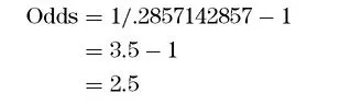
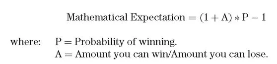
MATHEMATICAL EXPECTATION

At this point it is necessary to understand the concept of mathematical expectation, sometimes known as the player’s edge (if positive to the player) or the house’s advantage (if negative to the player):

(1.03)

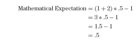
So, if you are going to flip a coin and you will win $2 if it comes up heads, but you will lose $1 if it comes up tails, the mathematical expectation per flip is:

In other words, you would expect to make 50 cents on average each flip.

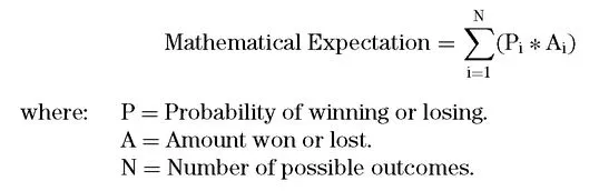
This formula just described will give us the mathematical expectation for an event that can have two possible outcomes. What about situations where there are more than two possible outcomes? The next formula will give us the mathematical expectation for an unlimited number of outcomes. It will also give us the mathematical expectation for an event with only two possible outcomes such as the 2 for 1 coin toss just described. Hence, it is the preferred formula.

(1.03a)

The mathematical expectation is computed by multiplying each possible gain or l...

Table of contents

• Title Page
• Copyright Page
• Preface
• Introduction
• PART I - Theory
• PART II - Practice
• Postscript
• Index