Mathematical Models

Jean-Michel Tanguy

• Publisher: Wiley-ISTE
• Year: 2012
• Print ISBN: 9781848211544
• eBook ISBN: 9781118587706
• Edition: 1
• Topic: Physical Sciences
• Subtopic: Hydrology

This series of five volumes proposes an integrated description of physical processes modeling used by scientific disciplines from meteorology to coastal morphodynamics. Volume 1 describes the physical processes and identifies the main measurement devices used to measure the main parameters that are indispensable to implement all these simulation tools. Volume 2 presents the different theories in an integrated approach: mathematical models as well as conceptual models, used by all disciplines to represent these processes. Volume 3 identifies the main numerical methods used in all these scientific fields to translate mathematical models into numerical tools. Volume 4 is composed of a series of case studies, dedicated to practical applications of these tools in engineering problems. To complete this presentation, volume 5 identifies and describes the modeling software in each discipline.

Chapter 1

Reminders on the Mechanical Properties of Fluids ¹

1.1. Laws of conservation, principles and general theorems

In this chapter, we will go back over the different theorems and principles of mechanics and thermodynamics and express them through Euler’s variable using the rules defined in previous volumes for a material domain.

1.1.1. Mass conservation, continuity equation

1.1.1.1. Mass conservation

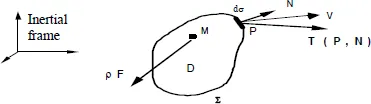
PRINCIPAL 1.1 (Figure 1.1). Mass in a material domain is conserved over the course of time.

Figure 1.1.

Taking D as a place for observation, noting that the material product for the mass of the domain is zero, we fully accept that the term for accumulation is balanced by the flow crossing the boundaries ∑.

We call

the surface effort at every point of ∑ of perpendicular angle

.

Note. As a rule, the perpendicular angle

will always be pulled toward the outside.

CLASSIFICATIONS. An integral as defined by volume is represented by ∫_D φdω, a surface integral ∫_D φdσ and a vector

.

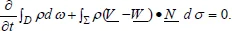
Faithful to Liebniz’ rule, the global equation is written as follows:

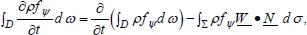
Liebniz’ rule: if D(t) is a deformable domain we can write:

therefore represents the localized velocity of displacement for all or part of the interface (boundary or component of the boundary) for D.

We notice that on the level of a mobile surface, the local flow

is zero by definition as the control’s surface sets the boundaries for the domain. This signifies that even if the fluid runs over the surface with a relative velocity above zero, it will not cross the surface, where the domain D is fixed:

represents the rate of accumulation (or loss) for mass in the domain.

represents the flow of mass crossing the boundaries of the domain.

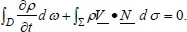
The conservation of mass for a domain is expressed as the void sum of a term of accumulation (or loss) of mass in the domain and as a fixed term representing flow of mass to the boundaries of the domain.

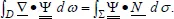
The term for flow is represented by

, using the following theorem.

Theorem for divergence

We will often have the need to pass between localized scripture to global scripture and vice versa. It is therefore important to be able to pass between integrals for volume and integrals for surface reciprocally. We therefore use the theorem of divergence:

.

This expression shows us that the integral for volume of a greater divergence is equal to the surface flow of the same size.

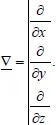
The pseudo-vector nabla is written as

It represents the gradient of the size we are considering. The point

represents the contracted product of two tensors (or the scalar product when applied to two vectors). The divergence is therefore equal to the scalar product of the operator nabla by the size being considered.

We can therefore consider that the divergence corresponds to the diffusion of a surface term on the inside of the liquid domain. In a more general way, every time we will meet a term for divergence in a localized equation, we will interpret it as the diffusion of an issued term from a surface action.

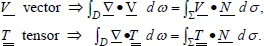
The theorem for divergence applies itself equally as well to vectors as to tensors:

A tensor is represented by

. It is said to be of second order if it is represented in the form of a 3 × 3 matrix. Its scalar product by a vector is a vector.

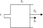
Figure 1.2.

EXAMPLE 1....

Table of contents

• Cover
• Title Page
• Copyright
• Introduction
• Chapter 1. Reminders on the Mechanical Properties of Fluids
• Chapter 2. 3D Navier-Stokes Equations
• Chapter 3. Models of the Atmosphere
• Chapter 4. Hydrogeologic Models
• Chapter 5. Fluvial and Maritime Currentology Models
• Chapter 6. Urban Hydrology Models
• Chapter 7. Tidal Model and Tide Streams
• Chapter 8. Wave Generation and Coastal Current Models
• Chapter 9. Solid Transport Models and Evolution of the Seabed
• Chapter 10. Oil Spill Models
• Chapter 11. Conceptual, Empirical and Other Models
• Chapter 12. Reservoir Models in Hydrology
• Chapter 13. Reservoir Models in Hydrogeology
• Chapter 14. Artificial Neural Network Models
• Chapter 15. Model Coupling
• Chapter 16. A Set of Hydrological Models
• List of Authors
• Index
• General Index of Authors
• Summary of the Other Volumes in the Series