Structural Equations with Latent Variables

Kenneth A. Bollen

• Publisher: Wiley-Interscience
• Year: 2014
• ISBN:
  9781118619032
• Edition: 1
• Topic: Mathematik
• Subtopic: Wahrscheinlichkeitsrechnung & Statistiken

Analysis of Ordinal Categorical Data Alan Agresti Statistical Science Now has its first coordinated manual of methods for analyzing ordered categorical data. This book discusses specialized models that, unlike standard methods underlying nominal categorical data, efficiently use the information on ordering. It begins with an introduction to basic descriptive and inferential methods for categorical data, and then gives thorough coverage of the most current developments, such as loglinear and logit models for ordinal data. Special emphasis is placed on interpretation and application of methods and contains an integrated comparison of the available strategies for analyzing ordinal data. This is a case study work with illuminating examples taken from across the wide spectrum of ordinal categorical applications. 1984 (0 471-89055-3) 287 pp. Regression Diagnostics Identifying Influential Data and Sources of Collinearity David A. Belsley, Edwin Kuh and Roy E. Welsch This book provides the practicing statistician and econometrician with new tools for assessing the quality and reliability of regression estimates. Diagnostic techniques are developed that aid in the systematic location of data points that are either unusual or inordinately influential; measure the presence and intensity of collinear relations among the regression data and help to identify the variables involved in each; and pinpoint the estimated coefficients that are potentially most adversely affected. The primary emphasis of these contributions is on diagnostics, but suggestions for remedial action are given and illustrated. 1980 (0 471-05856-4) 292 pp. Applied Regression Analysis Second Edition Norman Draper and Harry Smith Featuring a significant expansion of material reflecting recent advances, here is a complete and up-to-date introduction to the fundamentals of regression analysis, focusing on understanding the latest concepts and applications of these methods. The authors thoroughly explore the fitting and checking of both linear and nonlinear regression models, using small or large data sets and pocket or high-speed computing equipment. Features added to this Second Edition include the practical implications of linear regression; the Durbin-Watson test for serial correlation; families of transformations; inverse, ridge, latent root and robust regression; and nonlinear growth models. Includes many new exercises and worked examples. 1981 (0 471-02995-5) 709 pp.

CHAPTER ONE

Introduction

Most researchers applying statistics think in terms of modeling the individual observations. In multiple regression or ANOVA (analysis of variance), for instance, we learn that the regression coefficients or the error variance estimates derive from the minimization of the sum of squared differences of the predicted and observed dependent variable for each case. Residual analyses display discrepancies between fitted and observed values for every member of the sample.

The methods of this book demand a reorientation. The procedures emphasize covariances rather than cases.¹ Instead of minimizing functions of observed and predicted individual values, we minimize the difference between the sample covariances and the covariances predicted by the model. The observed covariances minus the predicted covariances form the residuals. The fundamental hypothesis for these structural equation procedures is that the covariance matrix of the observed variables is a function of a set of parameters. If the model were correct and if we knew the parameters, the population covariance matrix would be exactly reproduced. Much of this book is about the equation that formalizes this fundamental hypothesis:

(1.1)

In (1.1), ∑ (sigma) is the population covariance matrix of observed variables, θ (theta) is a vector that contains the model parameters, and ∑ (θ) is the covariance matrix written as a function of θ. The simplicity of this equation is only surpassed by its generality. It provides a unified way of including many of the most widely used statistical techniques in the social sciences. Regression analysis, simultaneous equation systems, confirmatory factor analysis, canonical correlations, panel data analysis, ANOVA, analy-sis of covariance, and multiple indicator models are special cases of (1.1).

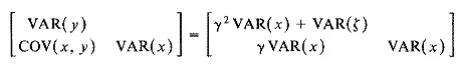
Let me illustrate. In a simple regression equation we have y = γx + ζ, where γ (gamma) is the regression coefficient, ζ (zeta) is the disturbance variable uncorrelated with x and the expected value of ζ, E(ζ), is zero.The y, x, and ζ are random variables. This model in terms of (1.1) is²

(1.2)

where VAR( ) and COV( ) refer to the population variances and covari- ances of the elements in parentheses. In (1.2) the left-hand side is 2, and the right-hand side is 2(6), with 0 containing γ, VAR(x), and VAR(ζ) as parameters. The equation implies that each element on the left-hand side equals its corresponding element on the right-hand side. For example, COV(x, y) = γVAR(x) and VAR(γ) = y² VAR(x) + VAR(ζ). I could modify this example to create a multiple regression by adding explanatory variables, or I could add equations and other variables to make it a simultaneous equations system such as that developed in classical econo- metrics. Both cases can be represented as special cases of equation (1.1), as I show in Chapter 4.

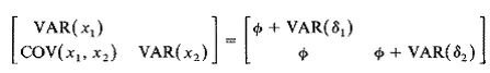
Instead of a regression model, consider two random variables, x_l and x₂, that are indicators of a factor (or latent random variable) called ξ (xi). The dependence of the variables on the factor is x₁ = ζ + δ₁ and x₂ = ξ + δ_2, where (delta) and δ₂ are random disturbance terms, uncorrelated with ξ and with each other, and E(δ₁ ) = E(δ₂) = 0. Equation (1.1) specializes to

(1.3)

where ϕ (phi) is the variance of the latent factor ξ. Here θ consists of three elements: ϕ, VAR(δ_X), and VAR(δ₂). The covariance matrix of the observed variables is a function of these three parameters. I could add more indicators and more latent factors, allow for coefficients ("factor loadings") relating the observed variables to the factors, and allow correlated disturbances creating an extremely general factor analysis model. As Chapter 7 demonstrates, this is a special case of the covariance structure equation (1.1).

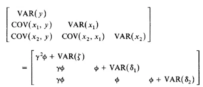
Finally, a simple hybrid of the two preceding cases creates a simple system of equations. The first part is a regression equation of y = γξ + ζ, where unlike the previous regression the independent random variable is unobserved. The last two equations are identical to the factor analysis example: x₁ = ξ+ δ₁ and x₂ = ξ+ δ₂. I assume that ζ, and δ₂ are uncorrected with ξ and with each other, and that each has an expected value of zero. The resulting structural equation system is a combination of factor analysis and regression-type models, but it is still a specialization of (1.1):

(1.4)

These examples foreshadow the general nature of the models I treat. My emphasis is on systems of linear equations. By linear, i mean that the relations between all variables, latent and observed, can be represented in linear structural equations or they can be transformed to linear forms.³ Structural equations that are nonlinear in the parameters are excluded. Nonlinear functions of parameters are, however, common in the covariance structure equation, ∑ = ∑(θ). For instance, the last example had three linear structural equations: y = γξ + ξ, x₁ = ξ + δ₁, and x₂ = ξ + δ₂. Each is linear in the variables and parameters. Yet the covariance structure (1.4) for this model shows that COV(x_1; y) = γϕ, which means that the COV(x_1,y) is a nonlinear function of γ and ϕ. Thus it is the structural equations linking the observed, latent, and disturbance variables that are linear, and not necessarily the covariance structure equations.

The term “structurai” stands for the assumption that the parameters are not just descriptive measures of association but rather that they reveal an invariant “causal” relation. I will have more to say about the meaning of “causality” with respect to these models in Chapter 3, but for now, let it suffice to say that the techniques do not “discover” causal relations. At best they show whether the causal assumptions embedded in a model match a sample of data. Also the models are for continuous latent and observed variables. The assumption of continuous observed variables is violated frequently in practice. In Chapter 9 I discuss the robustness of the standard procedures and the development of new ones for noncontinuous variables.

Structural equation models draw upon the rich traditions of several disciplines. I provide a brief description of their origins in the next section.

HISTORICAL BACKGROUND

Who invented general structural equation models? There is no simple answer to this question because many scholars have contributed to their development. The answer to this question is further complicated in that the models continue to unfold, becoming more general and more flexible. However, it is possible to outline various lines of research that have contributed to the evolution of these models.

My review is selective. More comprehensive discussions are available from the perspectives of sociology (Bielby and Hauser 1977), psychology (Bentler 1980; 1986), and economics (Goldberger 1972; Aigner et al. 1984). Two edited collections that represent the multidisciplinary origins of these techniques are the volumes by Goldberger and Duncan (1973) and Blalock ([1971] 1985). Other more recent collections are in Aigner and Goldberg (1977), Jöreskog and Wold (1982), the November 1982 issue of the Journal of Marketing Research, and the May–June 1983 issue of the Journal of Econometrics.

I begin by identifying three components present in today’s general structural equation models: (1) path analysis, (2) the conceptual synthesis of latent variable and measurement models, and (3) general estimation procedures. By tracing the rise of each component, we gain a better idea about the origins of these procedures.

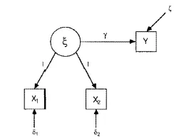
Let me consider path analysis first. The biometrician Sewall Wright (1918, 1921, 1934, 1960) is its inventor. Three aspects of path analysis are the path diagram, the equations relating correlations or covariances to parameters, and the decomposition of effects. The first aspect, the path diagram, is a pictorial representation of a system of simultaneous equations. It shows the relation between all variables, including disturbances and errors. Figure 1.1 gives a path diagram for the last example of the previous section. It corresponds to the equations:

where ξ, δ₁, and δ₂ are uncorrelated with each other and with ξ. Straight single-headed arrows represent one-way causal influences from the variable at the arrow base to the variable to which the arrow points. The implicit coefficients of one for the effects of ξ on x₁ and x₂ are made explicit in the diagram.

Figure 1.1 Path Diagram Example

Using the path diagram, Wright proposed a set of rules for writing the equations that relate the correlations (or covariances) of variables to the model parameters; this constitutes the second aspect of path analysis. The equations are equivalent to covariance structure equations, an example of which appears in (1.4). He then proposed solving these equations for the unknown parameters, and substituting sample correlations or covariances for their population counterparts to obtain parameter estimates.

The third aspect of path analysis provides a means to distinguish direct, indirect, and total effects of one variable on another. The direct effects are those not mediated by any other variable; the indirect effects operate through at least one intervening variable, and the total effects is the sum of direct sind all indirect effects.⁴

Wright’s applications of path analysis proved amazing. His first article in 1918 was in contemporary terms a factor analysis in which he formulated and estimated a model of the size components of bone measurements. This was developed without knowledge of Spearman’s (1904) work on factor analysis (Wright 1954, 15). Unobserved variables also appeared in some of his other applications. Goldberger (1972) credits Wright with pioneering the estimation of supply and demand equations with a treatment of identification and estimation more general than econometricians writing at the same time. His development of equations for covariances of variables in terms of model parameters is the same as that of (1.1), ∑ = ∑(θ), except that he developed these equations from path diagrams rather than the matrix methods employed today.

With all these accomplishments it is surprising that social scientists and statisticians did not pay more attention to his work. As Ben tier (1986) documents, psychometrics only flirted (e.g., Dunlap and Cureton 1930; Englehart 1936) with Wright’s path analysis. Goldberger (1972) notes the neglect of econometricians and statisticians with a few exceptions (e.g., Fox 1958; Tukey 1954; Moran 1961; Dempster 1971). Wright’s work also was overlooked in sociology until the 1960s. Partially in reaction to work by Simon (1954), Tukey (1954), and Turner and Stevens (1959), sociologists such as Blalock (1961, 1963, 1964), Boudon (1965), and Duncan (1966) saw the potential of path analysis and related “partial-correlation” techniques as a means to analyze nonexperimental data. Following these works, and particularly following Duncan’s (1966) expository account, the late 1960s and early 1970s saw many applications of path analysis in the sociological journals. The rediscovery of path analysis in sociology diffused to political science and several other social science disciplines. Stimulated by work in sociology, Werts and Linn (1970) wrote an expository treatment of path analysis, but it was slow to catch on in psychology.

The next major boost to path analysis in the social sciences came when Jöreskog (1973), Keesing (1972), and Wiley (1973), who developed very general structural equation models, incorporated path diagrams and other features of path analysis into their presentations. Researchers know these techniques by the abbreviation of the JKW model (Bentler 1980), or more commonly as the LISREL model. The tremendous popularity of the LISREL model has facilitated the spread of path analysis. Path analysis has evolved over the years. Its present form has some elaboration in the symbols employed in path diagrams, has equations relating covariances to parameters that are derived with matrix operations rather than from “reading” the path diagram, and has a more refined and clearly defined decomposition of direct, indirect, and total effects (see, e.g., Duncan 1971; Alwin and Hauser 1975; Fox 1980; Graff and Schmidt 1982). But the contributions of Wright’s work are still clear.

In addition to path analysis, the conceptual synthesis of latent variable and measurement models was essential to contemporary structural equation techniques. The factor analysis tradition spawned by Spearman (1904) emphasized the relation of latent factors to observed variables. The central concern was on what we now call the measurement model. The structural relations between latent variables other than their correlation (or lack of correlation) were not examined. In econometrics the focus was the structural relation between observed variables with an occasional reference to error-in-the-variable situations.

Wright’s path analysis examples demonstrated that econometric-type models with variables measured with error could be identified and estimated. The conceptual synthesis of models containing structurally related latent variables and more elaborate measurement models was developed extensively in sociology during the 1960s and early 1970s. For instance, in 1963 Blalock argued that sociologists should use causal models containing both indicators and underlying variables to make inferences about the latent variables based on the covariances of the observed indicators. He suggested that observed variables can be causes or effects of latent variables or observed variables can directly affect each other. He contrasted this with the restrictive implicit assumptions of factor analysis where all indicators are viewed as effects of the latent variable. Duncan, Haller, and Portes (1968) developed a simultaneous equation model of peer influences on high school students’ ambitions. The model included two latent variables reciprocally related, multiple indicators of the latent variables, and several background characteristics that directly affected the latent variables. Heise (1969) and others applied path analysis to separate the stability of latent variables from the reliability of measures.

This and related work in sociology during the 1960s and early 1970s demonstrated the potential of synthesizing econometric-type models with latent rather than observed variables and psychometric-type measurement models with indicators linked to latent variables. But their approach was by way of examples; they did not establish a general model that could be applied to any specific problems. It awaited the work of Jöreskog (1973), Keesing (1972), and Wiley (1973) for a practical general model to be proposed. Their models had two parts. The first was a latent variable model that was similar to the simultaneous equation model of econometrics except that all variables were latent ones. The second part was the measurement model that showed indicators as effects of the latent variables as in factor analyses. Matrix expressions for these models were presented so that they could apply to numerous individual problems. Jöreskog and Sörbom’s LISREL programs were largely responsible for popularizing these structural equation models, as were the numerous publications and applications of Jöreskog (e.g., 1967, 1970, 1973, 1977, 1978) and his collaborators.

Bentler and Weeks (1980), McArd...