Applied Survival Analysis

Regression Modeling of Time-to-Event Data

David W. Hosmer, Jr., Stanley Lemeshow, Susanne May

• Publisher: Wiley-Interscience
• Year: 2011
• Print ISBN: 9780471754992
• eBook ISBN: 9781118211588
• Edition: 2
• Topic: Mathematics
• Subtopic: Probability & Statistics
• Index: Mathematics

THE MOST PRACTICAL, UP-TO-DATE GUIDE TO MODELLING AND ANALYZING TIME-TO-EVENT DATA—NOW IN A VALUABLE NEW EDITION

Since publication of the first edition nearly a decade ago, analyses using time-to-event methods have increase considerably in all areas of scientific inquiry mainly as a result of model-building methods available in modern statistical software packages. However, there has been minimal coverage in the available literature to9 guide researchers, practitioners, and students who wish to apply these methods to health-related areas of study. Applied Survival Analysis, Second Edition provides a comprehensive and up-to-date introduction to regression modeling for time-to-event data in medical, epidemiological, biostatistical, and other health-related research.

This book places a unique emphasis on the practical and contemporary applications of regression modeling rather than the mathematical theory. It offers a clear and accessible presentation of modern modeling techniques supplemented with real-world examples and case studies. Key topics covered include: variable selection, identification of the scale of continuous covariates, the role of interactions in the model, assessment of fit and model assumptions, regression diagnostics, recurrent event models, frailty models, additive models, competing risk models, and missing data.

Features of the Second Edition include:

• Expanded coverage of interactions and the covariate-adjusted survival functions
• The use of the Worchester Heart Attack Study as the main modeling data set for illustrating discussed concepts and techniques
• New discussion of variable selection with multivariable fractional polynomials
• Further exploration of time-varying covariates, complex with examples
• Additional treatment of the exponential, Weibull, and log-logistic parametric regression models
• Increased emphasis on interpreting and using results as well as utilizing multiple imputation methods to analyze data with missing values
• New examples and exercises at the end of each chapter

Analyses throughout the text are performed using Stata® Version 9, and an accompanying FTP site contains the data sets used in the book. Applied Survival Analysis, Second Edition is an ideal book for graduate-level courses in biostatistics, statistics, and epidemiologic methods. It also serves as a valuable reference for practitioners and researchers in any health-related field or for professionals in insurance and government.

CHAPTER 1

Introduction to Regression Modeling of Survival Data

1.1 INTRODUCTION

Regression modeling of the relationship between an outcome variable and one or more independent (predictor) variable(s) is commonly employed in virtually all fields. The popularity of this approach is due to the fact that plausible models may be easily fit, evaluated, and interpreted. Statistically, the specification of a model requires choosing both systematic and error components. The choice of the systematic component involves an assessment of the relationship among the “average” of the outcome variable relative to specific levels of the independent variable(s). This may be guided by an exploratory analysis of the current data and/or past experience. The choice of an error component involves specifying the statistical distribution of what remains to be explained after the model is fit.

In an applied setting, the task of model selection is, to a large extent, based on the goals of the analysis and on the measurement scale of the outcome variable. For example, a clinician may wish to model the relationship among body mass index (BMI, kg/m²) and caloric intake and gender among teenagers seen in the clinics of a large health maintenance organization (HMO). A good place to start would be to use a model with a linear systematic component and normally distributed errors (i.e., the usual linear regression model). Suppose, instead, that the clinician decides to convert BMI into a 0 – 1 dichotomous variable (taking on the value 1 if BMI > 30) and assess its association with caloric intake and gender. In this case, the logistic regression model would be a good choice. The logistic regression model has a systematic component that is linear in the log-odds and has binomial/Bernoulli distributed errors. While there are many issues involved in the fitting, refinement, evaluation, and interpretation of each of these models, the same basic modeling paradigm would be followed in each scenario.

This basic modeling paradigm is commonly used in texts taking a data-based approach to either linear or logistic regression [e.g., Kleinbaum, Kupper, Muller and Nizam (1998) and Hosmer and Lemeshow (2000)]. In general we follow this same modeling paradigm in this text to motivate our study of regression models where the dependent variable measures the time to the occurrence of an event of interest. However, as we will see shortly, the fact that time to an event is the outcome of interest requires us to think carefully about what actually has been measured. Also the fact that time is a dynamic process provides challenges in formulating a model that are not present in settings where a typical linear or logistic regression model might be applied. In this spirit, we begin with an example.

Example

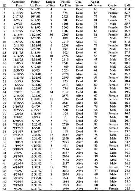
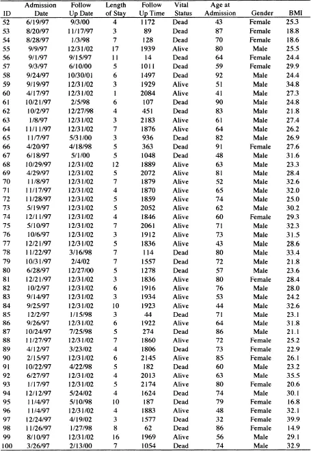
Throughout this book, we use a number of different data sets to illustrate the methods and provide grist for the exercises at the end of each chapter. Some, but not all, of these are described in Section 1.3. One is a subset of the data from the Worcester Heart Attack Study (WHAS) provided to us by its principal investigator, Dr. Robert J. Goldberg. Briefly, the goal of the WHAS is to study factors and time trends associated with long-term survival following acute myocardial infarction (MI) among residents of the Worcester, Massachusetts, Standard Metropolitan Statistical Area (SMSA). The study began in 1975 and has collected data approximately every other year, with the most recent cohort being subjects who experienced an MI in 2001. The main study has data on over 11,000 subjects, and we will focus our analyses on two samples from the main study. We present one such sample of 100 subjects in Table 1.1. These data are referred to as the WHAS 100 data in this text. Suppose our goal for the data in Table 1.1 is to study the effects of gender, age, and body mass index (kg/m²) at time of hospitalization for the MI on length of survival. Typical regression modeling questions might include: (1) Do women have a more favorable survival experience over time than men? (2) In what way do the age and BMI at admission affect survival over time? (3) Are the effects of age and BMI the same for men and women? Before we can discuss a regression model to address these questions, we need to consider what outcome variable we are going to model. If the outcome is time to an event, then what is the event and how do we define time to it? Suppose we consider the event of interest to be death from any cause following hospitalization for an MI and we define the time to it as the number of days from admission to the hospital until death. The next step in the regression modeling paradigm is to specify the systematic component. Because we have followed subjects over time, it seems logical that the systematic component should be the “mean” of this dynamic process and how it changes as a function of covariates. Prior experience in linear and logistic regression provides little guidance on how to do this. The first few chapters of this book are devoted to providing the necessary background and methods to begin to address this question as well as specification of the error component. The remainder of the text considers application of the methods to different time-to-event scenarios.

Returning to our outcome variable, each subject in Table 1.1 has a date recorded for when the last follow up occurred. Vital status reports whether the subject was dead or alive on that date. For those subjects who died, the reported date of death and the value presented for follow-up time is the actual value of the outcome of interest: survival time following hospitalization for an MI. For example, subject 5 in Table 1.1 was admitted to the hospital on February 9, 1995, and, 1205 days later, died on May 29, 1998. Subject 10 was admitted to the hospital on July 22, 1995, and was still alive at the time of his last follow up, December 31, 2001. For this subject, all we know is that his survival time exceeds the follow up time of 2719 days. Hence the observation of survival time is incomplete. The statistical term used to describe the process producing this type of incomplete observation is called “censoring” and the observation is referred to as being “censored.” In general, incomplete observation of time to an event can occur in several ways and we provide an overview of them in the next section. Methods for handling incompletely observed time-to-event data in regression models is a central theme in this text.

1.2 TYPICAL CENSORING MECHANISMS

We cannot discuss a censored observation until we have carefully defined an uncensored observation. This point may seem rather obvious, but in applied settings confusion, about censoring may not be due to the fact that some observations are incomplete but may instead be the result of an unclear definition of survival time.¹ The observation of survival time has two components that must be unambiguously defined: a beginning point (i.e., when the “clock starts”) and an endpoint that is reached when the event of interest occurs (i.e., when the “clock stops”). The point where analysis time, t, is zero is denoted t = 0 . In the WHAS example, observation began on the day a subject was admitted to the hospital following an MI. In a randomized clinical trial, observation of survival time usually begins on the day a subject is randomized to receive one of the treatment protocols. In an occupational exposure study, t = 0 may be the day a subject began work at a particular plant. In some applications, the best t = 0 point may not be obvious. For example, in the WHAS study, other beginning points might be the date of discharge from the hospital or the actual moment that the MI occurred. Observation may end at the time when a subject literally “dies” from the disease of interest, or it may end upon the occurrence of some other non-fatal, well-defined, condition such as meeting clinical criteria for remission of a cancer. The survival time is the distance on the time scale between these two points.

Table 1.1 Study ID, Admission Date, Follow Up Date, Length of Hospital Stay, Follow Up Time (Days), Vital Status at Follow Up, Age at Admission (Years), Gender, and Body Mass Index (kg/m²) (BMI) for 100 Subjects in the Worcester Heart Attack Study

In practice, a value of time is obtained by calculating the number of days (or months, or years, etc.) between two calendar dates. Table 1.1 shows the admission date and the follow up date for the subjects in this sample from the WHAS study. Most statistical software packages have functions that allow the user to manipulate calendar dates in a manner similar to other numeric variables. They do this by creating a numeric value for each calendar date, which is defined as the number of days from some predetermined reference date. For example, the reference date used by most, if not all, packages is January 1, 1960. Subject 5 entered the study on February 9, 1995, which is 12,823 days after the reference date, and died May 29, 1998, which is 14,028 days after the reference date. The interval between these two dates is 14,028 – 12,823 = 1,205 days. The number of days can be converted into the number of months by dividing by 30.4375 = (365.25/12). Thus, the survival time in months for subject 5 is 39.589 =(l,205 / 30.4375). It is common, when reporting results in tabular form, to round months to the nearest whole number, e.g., 40 months. The level of precision used in reporting and analyzing survival time should depend on the particular application.

Two mechanisms can lead to incomplete observation of time: censoring and truncation. A censored observation is one whose value is incomplete due to factors that are random for each subject. A truncated observation is incomplete due to a selection proce...

Table of contents

• Cover Page
• Title Page
• Seriestitle Page
• Copyright Page
• dedication
• Preface
• 1: Introduction to Regression Modeling of Survival Data
• 2: Descriptive Methods for Survival Data
• 3: Regression Models for Survival Data
• 4: Interpretation of a Fitted Proportional Hazards Regression Model
• 5: Model Development
• 6: Assessment of Model Adequacy
• 7: Extensions of the Proportional Hazards Model
• 8: Parametric Regression Models
• 9: Other Models and Topics
• Appendix 1: The Delta Method
• Appendix 2: An Introduction to the Counting Process Approach to Survival Analysis
• Appendix 3: Percentiles for Computation of the Hall and Wellner Confidence Band
• References
• Index