![]()
Chapter 1
Introduction to Inverse Problems in Imaging and Vision 1
The concept of an inverse problem is now a familiar concept to most scientists and engineers, particularly in the field of signal and image processing. In a nutshell, it involves the estimation of an unknown quantity, a mono-or multi-variate function f (r), starting from another observable quantity g(s) which is linked to it through a mathematical relationship known as the forward model. The main difficulty is that often such problems are ill posed [HAD 01]. The basic tools are therefore the theory of regularization [TIK 63, TIK 76] and its probabilistic counterpart of Bayesian estimation [HAN 83, TAR 82]. An earlier book on the subject in this same series, entitled Bayesian Approach to Inverse Problems [IDI 08], presents the basis of inversion methods, whether they be deterministic or probabilistic. However, the formulation of problems encountered in other communities in terms of an inverse problem, particularly in computer vision, as well as recent advances concerning inversion methods in imaging systems, prompted us to produce this book.
These days, in most imagery techniques, the aim is not only to construct images, but also to directly access the geometric characteristics of those images. This is why the main objective of this book is to focus on imagery and vision problems for which the problem can clearly be written in terms of an inverse problem. In the inverse problem an estimate for a function f (r) and its geometrical attributes is sought, in other words its contours q(r) or labels for its regions z(r) are to be determined from the observation g(s), which is linked to f (r) through what is known as the forward model.
The links between f(r) and g(s), on one hand, and between f(r) and its geometrical attributes q(r) and z(r) on the other hand, will be specified later. The main object of this introductory chapter is to present examples of inverse problems with different forward models and the bases of inversion methods.
1.1. Inverse problems
The unknown function f(r) and the observable function g(s) will not necessarily be defined in the same space. In fact, r and s can represent a position in space (x in 1D, (x, y) in 2D or (x, y, z) in 3D) or even a coordinate (x, y, z, t) in space-time or (x, y, z, λ) in space-wavelength (4D), etc. The two spaces may have the same dimensions, as is the case in image restoration, or different dimensions, as is the case for tomographic reconstruction.
The link between
f(
r) and
g(
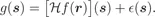
s) is described, in the most general case, by an operator
known as the
forward operator which, when applied to the function
f(
r), gives:
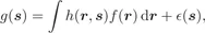
This equation is also known as the observation equation. In most cases, this relationship is not linear. However, a linear approximation can often be found which makes it possible to solve the problem more easily. In the case of a linear operator we have:
where h(r,s) represents the response of the measurement system.
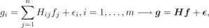
At this point, we should note that we are very often working in finite dimensions, and consequently we must discretize this equation. It is then easy to show that, in the general case, the discretized form of this equation can be written:
where, in the case of discretization using a simple lattice, we have
g i =
g(
s i),
i =
(
s i),
fj =
f(
rj ) and
H ij =
h(
rj , s i). In a more general ...