![]()
Chapter 1
Time Series Data: Examples and Basic Concepts
1.1 Introduction
In many fields of study, data is collected from a system (or as we would also like to call it a process) over time. This sequence of observations generates a time series such as the closing prices of the stock market, a country's unemployment rate, temperature readings of an industrial furnace, sea level changes in coastal regions, number of flu cases in a region, inventory levels at a production site, and so on. These are only a few examples of a myriad of cases where time series data is used to better understand the dynamics of a system and to make sensible forecasts about its future behavior.
Most physical processes exhibit inertia and do not change that quickly. This, combined with the sampling frequency, often makes consecutive observations correlated. Such correlation between consecutive observations is called autocorrelation. When the data is autocorrelated, most of the standard modeling methods based on the assumption of independent observations may become misleading or sometimes even useless. We therefore need to consider alternative methods that take into account the serial dependence in the data. This can be fairly easily achieved by employing time series models such as autoregressive integrated moving average (ARIMA) models. However, such models are usually difficult to understand from a practical point of view. What exactly do they mean? What are the practical implications of a given model and a specific set of parameters? In this book, our goal is to provide intuitive understanding of seemingly complicated time series models and their implications. We employ only the necessary amount of theory and attempt to present major concepts in time series analysis via numerous examples, some of which are quite well known in the literature.
1.2 Examples of Time Series Data
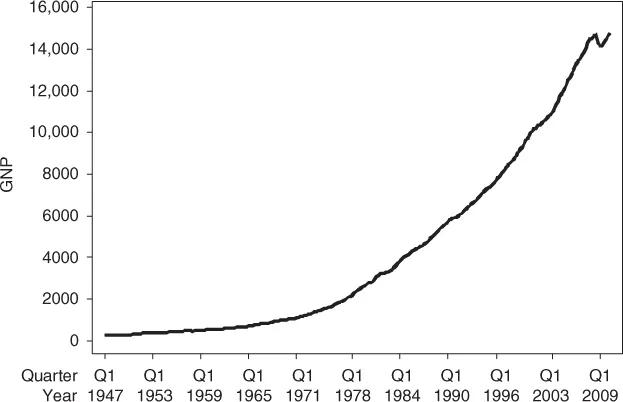
Examples of time series can be found in many different fields such as finance, economics, engineering, healthcare, and operations management, to name a few. Consider, for example, the gross national product (GNP) of the United States from 1947 to 2010 in Figure 1.1 where GNP shows a steady exponential increase over the years. However, there seems to be a “hiccup” toward the end of the period starting with the third quarter of 2008, which corresponds to the financial crisis that originated from the problems in the real estate market. Studying such macroeconomic indices, which are presented as time series, is crucial in identifying, for example, general trends in the national economy, impact of public policies, or influence of global economy.
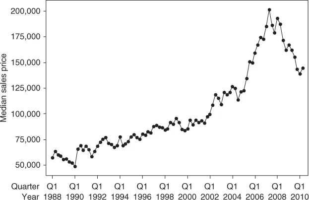
Speaking of problems with the real estate market, Figure 1.2 shows the median sales prices of houses in the United States from 1988 to the second quarter of 2010. One can argue that the signs of the upcoming crisis could be noticed as early as in 2007. However, the more crucial issue now is to find out what is going to happen next. Homeowners would like to know whether the value of their properties will fall further and similarly the buyers would like to know whether the market has hit the bottom yet. These forecasts may be possible with the use of appropriate models for this and many other macroeconomic time series data.
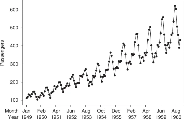
Businesses are also interested in time series as in inventory and sales data. Figure 1.3 shows the well-known number of airline passengers data from 1949 to 1960, which will be discussed in greater detail in Chapter 5. On the basis of the cyclical travel patterns, we can see that the data exhibits a seasonal behavior. But we can also see an upward trend, suggesting that air travel is becoming more and more popular. Resource allocation and investment efforts in a company can greatly benefit from proper analysis of such data.
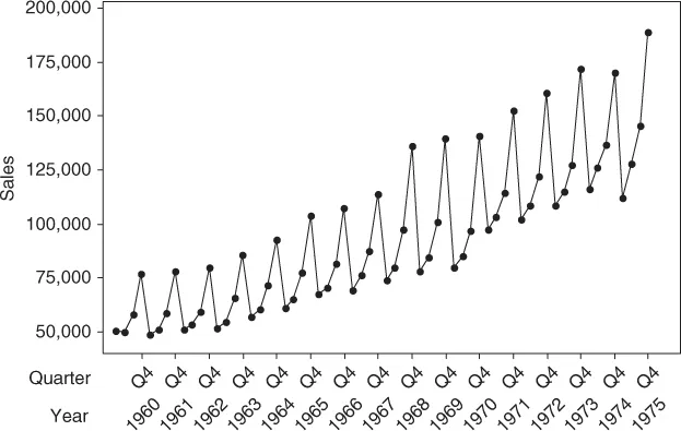
In Figure 1.4, the quarterly dollar sales (in $1000) data of Marshall Field & Company for the period 1960 through 1975 also shows a seasonal pattern. The obvious increase in sales in the fourth quarter can certainly be attributed to Christmas shopping sprees. For inventory problems, for example, this type of data contains invaluable information. The data is taken from George Foster's Financial Statement Analysis (1978), where Foster uses this dataset in Chapter 4 to illustrate a number of statistical tools that are useful in accounting.
In some cases, it may also be possible to identify certain leading indicators for the variables of interest. For example, building permit applications is a leading indicator for many sectors of the economy that are influenced by construction activities. In Figure 1.5, the leading indicator is shown in the top panel whereas the sales data is given at the bottom. They exhibit similar behavior; however, the important task is to find out whether there exists a lagged relationship between these two time series. If such a relationship exists, then from the current and past behavior of the leading indicator, it may be pos...