Monitoring and Modeling the Deepwater Horizon Oil Spill

A Record Breaking Enterprise

Yonggang Liu, Amy MacFadyen, Zhen-Gang Ji, Robert H. Weisberg, Yonggang Liu, Amy MacFadyen, Zhen-Gang Ji, Robert H. Weisberg

• Publisher: American Geophysical Union
• Year: 2013
• Print ISBN: 9780875904856
• eBook ISBN: 9781118671825
• Edition: 1
• Topic: Physical Sciences
• Subtopic: Geophysics

Published by the American Geophysical Union as part of the Geophysical Monograph Series, Volume 195. Monitoring and Modeling the Deepwater Horizon Oil Spill: A Record-Breaking Enterprise presents an overview of some of the significant work that was conducted in immediate response to the oil spill in the Gulf of Mexico in 2010. It includes studies of in situ and remotely sensed observations and laboratory and numerical model studies on the four-dimensional oceanographic conditions in the gulf and their influence on the distribution and fate of the discharged oil. Highlights of the book include discussions of the following: immediate responses to the Deepwater Horizon oil spill using Integrated Ocean Observing System resources; monitoring the surface and subsurface oil using satellites, aircraft, vessels, and AUVs; mapping the oceanographic conditions using satellites, aircraft, vessels, drifters, and moorings; modeling the spreading of surface oil trajectories and the three-dimensional dispersal of subsurface hydrocarbon plumes; oil spill risk analyses and statistical studies on the fate of the oil; and laboratory investigation of ocean stratification related to subsurface plumes. This book will be of value to scientists interested in the Deepwater Horizon oil spill, the Gulf of Mexico, and the potential for conveyance of oil spilled in the Gulf of Mexico to the North Atlantic. A more technical audience may include those interested in oil spill detection, trajectory model forecasting, and risk analyses and those with an interest in applied oceanography, including scientists, engineers, environmentalists, natural and living marine resource managers and students within academic institutions, agencies, and industries who are involved with the Gulf of Mexico and other regions with offshore oil and gas exploration and production.

Airborne Ocean Surveys of the Loop Current Complex From NOAA WP-3D in Support of the Deepwater Horizon Oil Spill

Lynn K. Shay,¹ Benjamin Jaimes,¹ Jodi K. Brewster,¹ Patrick Meyers,¹ E. Claire McCaskill,¹ Eric Uhlhorn,² Frank Marks,² George R. Halliwell Jr.,³ Ole Martin Smedstad,⁴ and Patrick Hogan⁵

¹ Rosenstiel School of Marine and Atmospheric Science, Division of Meteorology and Physical Oceanography, University of Miami, Miami, Florida, USA.

² NOAA Atlantic Oceanographic and Meteorological Laboratory, Hurricane Research Division, Miami, Florida, USA.

³ NOAA Atlantic Oceanographic and Meteorological Laboratory, Physical Oceanography Division, Miami, Florida, USA.

⁴ QinetiQ North America, Stennis Space Center, Mississippi, USA.

⁵ Naval Research Laboratory, Stennis Space Center, Mississippi, USA.

At the time of the Deepwater Horizon oil rig explosion, the Loop Current (LC), a warm ocean current in the Gulf of Mexico (GoM), extended to 27.5°N just south of the rig. To measure the regional scale variability of the LC, oceanographic missions were flown on a NOAA WP-3D research aircraft to obtain ocean structural data during the spill and provide thermal structure profiles to ocean forecasters aiding in the oil spill disaster at 7 to 10 day intervals. The aircraft flew nine grid patterns over the eastern GoM between May and July 2010 deploying profilers to measure atmospheric and oceanic properties such as wind, humidity, temperature, salinity, and current. Ocean current profilers sampled as deep as 1500 m, conductivity, temperature, and depth profilers sampled to 1000 m, and bathythermographs sampled to either 350 or 800 m providing deep structural measurements. Profiler data were provided to modeling centers to predict possible trajectories of the oil and vector ships to regions of anomalous signals. In hindcast mode, assimilation of temperature profiles into the Hybrid Coordinate Ocean Model improved the fidelity of the simulations by reducing RMS errors by as much as 30% and decreasing model biases by half relative to the simulated thermal structure from models that assimilated only satellite data. The synoptic snapshots also provided insight into the evolving LC variability, captured the shedding of the warm core eddy Franklin, and measured the small-scale cyclones along the LC periphery.

1. INTRODUCTION

On 20 April 2010, the Deepwater Horizon (DwH) oil rig, located at a water depth of ∼1675 m on the northern continental slope of the Gulf of Mexico (GoM) adjacent to the DeSoto Canyon, exploded causing a major oil spill that lasted for 107 days until it was capped on 15 July. At the time of the explosion, the Loop Current (LC) extended north of its mean position where the average maximum northward extension of the LC intrusion is 26.2°N [Leben, 2005; Vukovich, 2007]. The northern edge of the LC extended to ∼27.5°N during the first few weeks of the oil spill based on the sea surface height field where surface geostrophic velocities exceeded 1.5 m s⁻¹.

The anticyclonically rotating LC generally has two forms: a retraction phase where the LC makes a direct link from the Yucatan Straits to the Florida Straits as observed during 2002 [Shay and Uhlhorn, 2008], and a bulging phase, where the LC meanders deep into the GoM before exiting to the east through the Florida Straits [Nof, 2005]. Surrounding a bulging LC is a complex eddy field including both cyclonic and anticyclonically rotating eddies [Schmitz, 2005; Vukovich, 2007]. The larger anticyclonically rotating warm core eddies (WCE) have a vertical scale of O(1000 m) with diameters between 200 and 400 km [Mooers and Maul, 1998]. By contrast, smaller-scale cyclonically rotating cold core eddies (CCE) are found along the periphery of the LC [Hamilton, 1992; Zavala-Hidalgo et al., 2003] and are vitally important in the shedding of the WCEs from the LC through current instabilities [Schmitz, 2005; Chérubin et al., 2005]. That is, the LC bulge eventually may pinch off and form a WCE, which moves to the west to southwest at speeds of a few km d⁻¹ [Elliot, 1982; Sturges and Leben, 2000]. Because the LC path was characteristic of this bulging phase during the spill similar to that observed during Hurricanes Katrina and Rita [Scharroo et al., 2005; Jaimes and Shay, 2009], a possibility existed for oil to be transported from the northern GoM to the southern tip of Florida and into the Florida Current and Gulf Stream, potentially impacting the ecosystems of the Florida Keys and the southeast coast of Florida.

During the summer of 2010, the bulging LC intrusion was followed by a series of attachments and reattachments of WCE Franklin that influenced the ocean current structure south of the rig [Hamilton et al., this volume; Walker et al., this volume]. As shown in Figure 1, smaller-scale cyclonic eddies were located along the northern extent of the LC that impacted the circulation patterns near the rig during most of the observational period and facilitated the entrainment of oil into the LC [Walker et al., this volume; Liu et al., this volume].

In this broader context, emergency responders and modeling teams were concerned the LC and its complex eddy field would be a major mechanism for oil transport throughout the GoM. In addition to satellite measurements for the surface layer, near real-time information on LC properties using various in situ platforms was needed to monitor its position and subsurface ocean structure because this spill was subsurface. A NOAA research aircraft flew oceanographic survey missions to provide synoptic oceanic and atmospheric measurements to provide guidance to the ocean forecast community and emergency responders on the LC variability. These flights provided near real-time temperature profile data over 7 to 10 days intervals for assimilation into ocean models at forecasting centers such as the Naval Oceanographic Office to predict the circulation and potential pathways of the oil. These measurements provided data to vector ships such as the NOAA R/V Nancy Foster to regions of mesoscale variability and were used to evaluate satellite-based products such as oceanic heat content [Mainelli et al., 2008]. In this manuscript, the oceanographic surveys are described in section 2 including a brief description of the sensor packages and their respective measurement uncertainties. Section 3 discusses the observed variability from the oceanic and atmospheric profilers and salient results such as the subsurface thermostad observed in the northwestern part of the grid as well as comparisons to satellite-derived isotherm depths (20°C isotherm depth: H₂₀) from altimetry. Section 4 focuses on twin assimilation experiments that ingest and deny the thermal structure data from the oceanographic surveys into the Hybrid Coordinate Ocean Model (HYCOM). The results are summarized in section 5 with concluding remarks with an emphasis on future research efforts.

2. AIRBORNE OCEAN SURVEYS

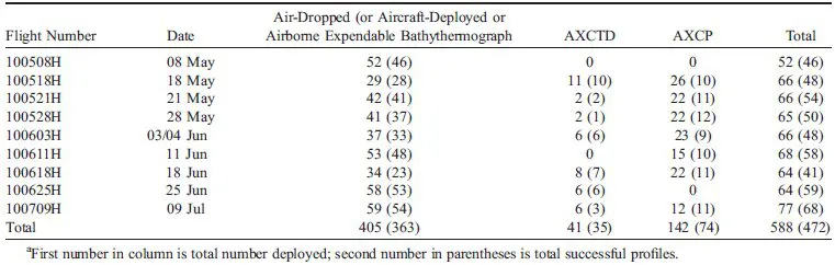
Nine flights on NOAA’s WP-3D Orion aircraft were conducted between 8 May and 9 July 2010 (Figure 1) over the region extending from just south of the DwH rig southward over the LC and associated frontal eddies. Expendable probes measured atmospheric and oceanic properties every 7 to 10 days over the northeastern GoM. In total, 588 airborne profilers were deployed (Table 1), specifically 405 bathythermographs (airborne expendable bathythermographs (AXBT)), 142 current-temperature profilers (airborne expendable current profiler (AXCP)), and 41 conductivity-temperature-depth profilers (airborne expendable conductivity temperature and depth profiler (AXCTD)). The configuration of the aircraft sampling pattern was similar to that used during NOAA’s Hurricane Intensity Forecast Experiments [Rogers et al., 2006]. During the first seven flights, failure rates for the AXCPs were unusually high compared to other experiments. These hardware problems included radio frequency (RF) transmission where either the transmitters did not turn on (e.g., no RF quieting) or the RF signals were too low to be detected. These problems were resolved during the final missions where the failure rate was less than 10%. Despite these problems with the AXCPs, the thermal structure over the LC system was well resolved from the aircraft measurements.

Figure 1. Eight of the nine flight tracks of the WP-3D and profiler drop points overlaid on absolute sea surface height (SSH, color) and altimetry-derived geostrophic currents (arrows). Yellow triangles are for the position of the DwH rig; red and white circles are for good and bad profilers, respectively. The absolute SSH (or η) and surface geostrophic currents were derived from: Daily maps from satellite-based measurements of the surface height anomaly (SHA) from NASA Jason-1 and Jason-2, and European Space Agency (ESA) Envisat from May to July 2010; η was estimated for the entire GoM by adding the SHA fields to the Combined Mean Dynamic Topography Rio05 [Rio and Hernandez, 2004], representing the mean sea surface height above a geoid computed over a 7 year period (1993–1999); and surface geostrophic flows (V_g = U_gi + V_gj) from the horizontal gradients in η (U_g = −(g/f )∂η/∂y, V_g = (g/f )∂η/∂x, where f is the Coriolis parameter). Note the maximum surface current vector is 2 m s⁻¹. Dark blue and red shades of SSH are for cyclonic and anticyclonic geostrophic features, respectively.

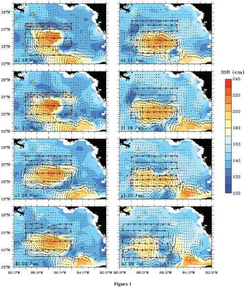
Table 1. Number and Type of Expendable Profilers Deployed During the DwH Oil Spill ^a

2.1. Flight Tracks

Research flights on the NOAA aircraft departed from Mac-Dill Air Force Base and had durations of 8 to 10 h. During a typical mission, the aircraft flew at ∼1700 m at an indicated air speed between 90 and 95 m s⁻¹ for optimal deployment of the expendable probes. Ocean profilers were deployed in lawnmower style grids (see Figure 1). These flights sampled essentially the same grid points, to as deep as 1500 m, to provide the evolving oceanic variability of the LC associated with the potential shedding of Eddy Franklin. Atmospheric dropsondes [Hock and Franklin, 1999] were deployed in the center of the flight tracks with others deployed along the edges of the LC over the strong frontal zones. On several flights, AXCPs and AXCTDs were deployed at the same points as AXBTs to compare T(z) profiles over the upper 350 m.

During the first two legs of the 8 May 2010 flight (not shown), the aircraft was flown at 350 m to be below the cloud deck and avoid deploying profilers on other aircraft or containment vessels. Five legs of the grid were spaced at 0.5° intervals (∼55 km) from 28.4°N to 26.5°N spanning 89°W to 84.5°W. On the sixth drop (86.5°W, 28.3°N), oil globs appeared and then organized into a slick as the aircraft flew westward toward the DwH Site. During the remaining legs of the grid, the flight level was 1700 m. Oil was not seen again until the final leg of our grid where the aircraft traveled due north along 88°W into the main oil spill area. The northern edge of the grid was limited to 28.3°N due to the restricted no-fly zone surrounding the DwH spill.

After the initial flight, the grid was expanded southward to encompass more of the eastern GoM and capture the oceanic variability in the frontal CCEs, which facilitate WCE shedding through baroclinic and barotropic instability (e.g., vertical and horizontal current shear, respectively). More oil slicks were observed in the CCE located at 25°N 85.5°W, and a rainbow oil sheen was observed at 24°N, 85°W as well as along the northwestern part of the two northernmost legs (Figure 1a). Prior to flying over the final transect, the aircraft dropped to ∼1000 m and proceeded northeastward to fly over the well site to calibrate the Stepped Frequency Microwave Radiometer (SFMR) [Uhlhorn et al., 2007] and the downward-looking infrared radiometer thermometer by acquiring data on sea surface properties such as sea surface temperatures (SST) and brightness temperatures. The aircraft flew over brown oil, rainbow and dull sheens, as well as the silver sheens where wind rows of red/orange emulsion surrounded the site as reported in the U.S. Coast Guard (USCG) HC-144 images.

Flight tracks for 18, 21, and 28 May 2010 were similar (Figures 1a–1c) with four transects spaced at 1° intervals in latitude (∼110 km) between 24°N and 27°N spanning longitudes from 89°W to 85°W at 0.5° resolution. Along the last two transects at 27°N and 27.5°N, expendable profilers were deployed at 0.25° resolution in the area located due south of the no-fly zone that was sampled during the 8 May flight. On 21 May 2010, additional higher resolution measurements (0.25°) were acquired through the CCE at 25°N, 85.5°W. Along the last two legs from 27°N to 27.5°N, expendable profilers were once again deployed at 0.25° resolution in the area located due south of the no-fly zone sampled during the 8May flight. Based on analyses from the 28May SFMRflight data over the oil slick, the brightness temperatures did not change across the thick oil slick and the sheen. This is good news for future hurricane flights because surface winds can be mapped during strong winds even when oil slicks are present.

Flights on 3 and 4 June 2010 (combined as 1 day in Figure 1d) deviated slightly from the typical flight plan. As on the 28 May flight, four of the six legs of the grid were spaced at 1° intervals in latitude (∼110 km) from 24.5°N to 27°N and spanning 89°W to 85°W with profiler deployments at 0.5° resolution. The last two transects were at 27.5°N and 28°N with similar spatial resolution. All but one leg of the grid was finished on 3 June 2010 as the NOAA aircraft landed in Baton Rouge that evening. On the morning of 4 June, the NOAA Administrator (Dr Jane Lubchenco) boarded the aircraft for an aerial view of the spill site, while the aircraft acquired radiometer data and deployed profilers along the northern transect (28°N) of the grid. The aircraft returned to Pascagoula, MS to refuel and for passengers to disembark from the aircraft. The aircraft returned to the northern transect, deployed six profilers, then returned to MacDill Air Force Base.

On 11 June 2010 (Figure 1e), t...

Table of contents

• Cover
• Contents
• Series Page
• Title Page
• Copyright
• Preface
• Introduction to Monitoring and Modeling the Deepwater Horizon Oil Spill
• NOAA’s Satellite Monitoring of Marine Oil
• A New RST-Based Approach for Continuous Oil Spill Detection in TIR Range: The Case of the Deepwater Horizon Platform in the Gulf of Mexico
• Studies of the Deepwater Horizon Oil Spill With the UAVSAR Radar
• Absolute Airborne Thermal SST Measurements and Satellite Data Analysis From the Deepwater Horizon Oil Spill
• A High-Resolution Survey of a Deep Hydrocarbon Plume in the Gulf of Mexico During the 2010 Macondo Blowout
• Analyses of Water Samples From the Deepwater Horizon Oil Spill: Documentation of the Subsurface Plume
• Evaluation of Possible Inputs of Oil From the Deepwater Horizon Spill to the Loop Current and Associated Eddies in the Gulf of Mexico
• Evolution of the Loop Current System During the Deepwater Horizon Oil Spill Event as Observed With Drifters and Satellites
• Impacts of Loop Current Frontal Cyclonic Eddies and Wind Forcing on the 2010 Gulf of Mexico Oil Spill
• Loop Current Observations During Spring and Summer of 2010:Description and Historical Perspective
• Airborne Ocean Surveys of the Loop Current Complex From NOAA WP-3D in Support of the Deepwater Horizon Oil Spill
• Trajectory Forecast as a Rapid Response to the Deepwater Horizon Oil Spill
• Tactical Modeling of Surface Oil Transport During the Deepwater Horizon Spill Response
• Surface Drift Predictions of the Deepwater Horizon Spill: The Lagrangian Perspective
• On the Effects of Wave-Induced Drift and Dispersion in the Deepwater Horizon Oil Spill
• Tracking Subsurface Oil in the Aftermath of the Deepwater Horizon Well Blowout
• Simulating Oil Droplet Dispersal From the Deepwater Horizon Spill With a Lagrangian Approach
• Oil Spill Risk Analysis Model and Its Application to the Deepwater Horizon Oil Spill Using Historical Current and Wind Data
• A Statistical Outlook for the Deepwater Horizon Oil Spill
• Possible Spreadings of Buoyant Plumes and Local Coastline Sensitivities Using Flow Syntheses From 1992 to 2007
• Subsurface Trapping of Oil Plumes in Stratification: Laboratory Investigations
• AGU Category Index
• Index