![]()
PART I
MODELING
![]()
1
INTRODUCTION
1.1 INTEGER PROGRAMMING
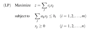
A linear programming problem (LP) is a class of the mathematical programming problem, a constrained optimization problem, in which we seek to find a set of values for continuous variables (x1, x2,…, xn) that maximizes or minimizes a linear objective function z, while satisfying a set of linear constraints (a system of simultaneous linear equations and/or inequalities). Mathematically, an LP is expressed as follows:
An integer (linear) programming problem (IP) is a linear programming problem in which at least one of the variables is restricted to integer values. In the past two decades, there has been an increasing use of an alternate term—mixed integer programming problem (MIP)—for LPs with integer restrictions on some or all of the variables. In this text, the terms IP and MIP may be used interchangeably unless there is a chance of confusion. For clarity, we shall use the term pure integer programming problem (or pure IP) to emphasize an IP whose variables are all restricted to be integer valued.
The term “programming” in this context means planning activities that consume resources and/or meet requirements, as expressed in the m constraints, not the other meaning—coding computer programs. The resources may include raw materials, machines, equipments, facilities, workforce, money, management, information technology, and so on. In the real world, these resources are usually limited and must be shared with several competing activities. Requirements may be implicitly or explicitly imposed. The objective of the LP/IP is to allocate the shared resources, and responsibility to meet requirements, to all competing activities in an optimal (best possible) manner.
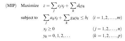
The term “programming problem” is sometimes replaced by program, for short. Thus, an integer programming problem is also called an integer program, and so are mixed integer program, pure integer program, and so on. Mathematically, an MIP is defined as
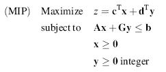
Note that all input parameters (cj, dk, aij, gik, bi) may be positive, negative, or zero. Using matrix notation, a mixed integer program may be expressed as
where m = number of constraints
n = number of continuous variables
p = number of integer variables
cT = (cj) is a row vector of n elements
dT = (dk) is a row vector of p elements
A = (aij) is an m × n matrix
G = (gik) is an m × p matrix
b = (bi) is a column vector of m constants (or right-hand-side column, rhs)
x = (xj) is a column vector of n continuous variables
y = (yk) is a column vector of p integer variables
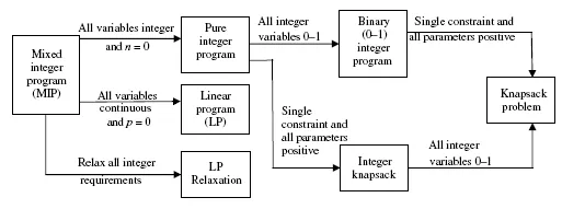
When n = 0, no continuous variables x are present and the MIP reduces to a pure IP. When p = 0, no integer-restricted variables y are present and the MIP reduces to a linear program. An LP is also obtained by relaxing (or ignoring) the integer requirements in a given MIP. Thus, the resulting LP is called the LP relaxation (of a given IP). Unlike the above-mentioned LP that contains only variables x, the LP relaxation contains both x and y variables and treats y as a vector of continuous variables.
An integer program in which the integer variables are restricted to be 0 or 1 is called a 0–1 (binary) integer program, or binary IP (BIP). A binary IP with a single ≤ linear constraint, whose objective function and constraint coefficients are all positive, is called a knapsack (or backpack) problem. An IP with a single constraint and all positive constraint coefficients is called an integer knapsack program, in which the values of an integer variable are not restricted to 0–1. In particular, an integer knapsack program is a knapsack program if all integer variables are restricted to be 0 or 1. Figure 1.1 depicts the relationships between various classes of MIPs under certain conditions. A box represents an IP class and an arrow represents the imposed condition(s) leading to a subclass from a class. There are many more subclasses than shown in this simple diagram, but the details of Figure 1.1 are adequate for this introductory chapter.
1.2 STANDARD VERSUS NONSTANDARD FORMS
Throughout this text, a mixed integer program will be said to be in standard form if (1) the objective function is maximized, (2) all the constraints are of ≤ form, (3) each integer variable is defined over consecutive integer numbers whose lower bound is 0 and upper bound infinity, and (4) each continuous variable is nonnegative with no finite upper bound.
Any MIP that does not conform to the conditions (1)–(4) is considered to be in nonstandard form, but may be converted to a standard one through simple mathematical manipulations. For ease of presentation, we shall use the standard form for the remainder of the text, except for special purposes. The following are various nonstandard forms that need to be converted:
- Minimization problem
- Inequality of ≥ form
- Equation (equality constraint)
- Unrestricted variable (continuous or integer)
- Variable with a positive or a negative lower bound
- Variable with a finite upper bound
If a given problem is a minimization problem, then it may be converted to an “equivalent” maximization problem. Two problems are considered equivalent if their optimal solutions are the same. Consider the given problem,
To convert to a standard form, we multiply the given objective function by –1 and change the minimization to the maximization as follows:
For example, we convert min z′ = 3x1 − 2x2 + 4x3 to max z = −3x1 + 2x2 − 4x3, and the new objective value becomes z = −z′.
If a given inequality is in ≥ form, we then convert it to the standard ≤ form by multiplying the inequality by −1 and reversing the direction of the inequality sign. For example, the inequality 6x1 − 5x2 + 3x3 ≥ 10 may be converted to − 6x1 + 5x2 − 3x3≤ − 10.
Converting an equation to the standard ≤ form requires two steps: (1) replace the equation by a pair of inequalities of opposite sense, and as before, (2) convert the inequality of ≥ form to the standard ≤ form. For example, we first convert −2x1 + 5x2 − 3x3 = 15 to the following two inequalities: −2x1 + 5x2 − 3x3 ≤ 15 and −2x1 + 5x2 − 3x3 ≥ 15. We then convert the nonstandard inequality by multiplying it by −1 and reversing the sign of the inequality to get the second standard inequality: 2x1 − 5x2 + 3x3≤ − 15.
If a continuous or an integer variable is unrestricted in sign (i.e., it can be negative, positive, or zero), then we may replace an unrestricted variable by the difference of two new variables,
and
, as follows:
Note ...