Wiley Finance

Capturing Systematic Sources of Active Equity Returns

Khalid Ghayur, Ronan G. Heaney, Stephen A. Komon, Stephen C. Platt, Stephen C. Platt

• Publisher: Wiley
• Year: 2010
• Print ISBN: 9780470610022
• eBook ISBN: 9780470632970
• Edition: 1
• Topic: Business
• Subtopic: Investments & Securities
• Index: Business

An informative guide offering new and innovative ways to think about active management and investing

ActiveBeta Indexes presents exciting new research that shows how above-market returns can be achieved in a low-cost, transparent, and efficient fashion. Active Betas reflect fundamental investment principles that have long been the foundation of active equity returns, but are commonly masqueraded as investment skill, or alpha. This groundbreaking book lifts the veil to uncover the common sources of active returns and reveals their beta-like properties.

Developed by leading investment practitioners at Westpeak Global Advisors, ActiveBeta Indexes introduces Active Beta sources and explains how the behavior of short- and long-term earnings growth gives rise to systematic sources of active equity returns.

• Details a new index framework and research findings that could change the face of active portfolio management
• Presents patent-pending innovations for constructing style indexes and informationally-efficient active portfolios
• Explores the historical performance of ActiveBeta Indexes

Wealth advisers, consultants, pensions and endowments, and other institutional investors will find the intellectual honesty of ActiveBeta Indexes a refreshing perspective on the active management industry. They will also find it a useful guide to a more strategic allocation of their risk and management fee budgets – a growing necessity in these challenging times.

SECTION Two

ActiveBeta Conceptual Framework

CHAPTER 3

Introducing Active Betas

In order to better define the investment styles of active managers and create style indexes that reflect what active style managers actually do, we need to develop a framework to explain what influences could give rise to common sources of active equity returns, that is, equity styles. In this chapter, we introduce Active Betas as the primary common sources of active equity returns. In Chapters 4 through 6, we develop further the concepts and relationships that provide the foundation for the proposed ActiveBeta Framework.

DEFINING ACTIVE BETAS

Many investors believe that markets are highly efficient and highly adaptive. In a highly efficient market, pure alpha could exist, but it should be difficult to find and require significant investment skill. In a highly adaptive market, a particular source of alpha, once discovered and documented, should lose its effectiveness over time as it becomes commoditized or is arbitraged away.

Yet, sources of positive active returns (returns in excess of the market), which do not require a high level of investment skill to capture, have been easily found. These include size (market capitalization), value (e.g., price-book value), momentum (relative returns), and so forth. Even more surprisingly, some sources of positive active returns have persisted over time despite the fact that they were discovered and documented decades ago.

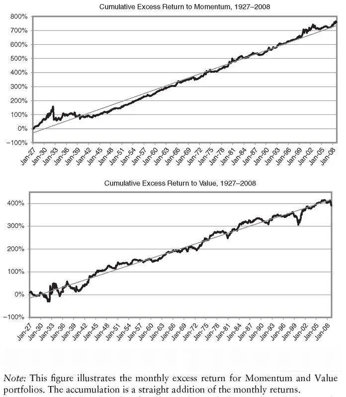
Consider Figure 3.1. It depicts the cumulative excess returns over cash generated by the Fama-French 12-month price momentum factor and the price-book value factor for U.S. stocks since 1927. These returns reflect the performance of long-short, market-neutral factor portfolios generated by subtracting the returns of high momentum and value stocks from the returns of low momentum and value stocks. From 1927 through 2008, a total of 82 years, momentum and value have provided significant excess returns, despite their well-known existence and straightforward definitions. It should be noted that since these excess returns are not adjusted for transaction costs, it appears that momentum, a high turnover strategy, has delivered better performance than value, a low turnover strategy. Once implementation costs are considered, the two strategies generate almost identical Sharpe ratios.

FIGURE 3.1 Performance of Fama-French Momentum and Value Factors for U.S. Stocks, 1927 through 2008

Source: Westpeak, based on data from Kenneth French (http://mba.tuck.dartmouth.edu/pages/faculty/ken.french/data_library.html ).

Interestingly, the value effect was documented as far back as 1977 by Basu. Value as an investment style gained greater industry-wide popularity after Fama and French published their research in 1992. Meanwhile, the success of medium-term momentum was documented by Jegadeesh and Titman in 1993. However, value and momentum have shown no evidence of losing their excess return generation capability since the 1990s, as depicted by the slope of the two lines in Figure 3.1.

How can these publicly documented excess returns coexist with a basic acceptance of the highly efficient and adaptive nature of equity markets? While many theories have been offered to explain the nature of momentum and value active returns (as we discuss in Chapter 6), our research provides some fresh insights on how to reconcile this conflict between core investment beliefs and observed facts. It highlights that simple and publicly known sources of active returns that persist over time emanate from systematic sources of active equity returns.

By “systematic” we mean a system that adheres to an intuitive, fundamental law, which gives rise to predictable and consistent behavior of the variables that drive stock prices, such as earnings and discount rates. This predictable behavior, when captured in appropriate investment strategies, gives rise to persistent sources of active equity returns.

A basic law characterizes the behavior of earnings (and discount rates) in open, competitive, free-market economies. That is, earnings for large groups of stocks cannot grow at above-average rates indefinitely. Competitive forces cause both prior fast and slow growers to revert toward the mean over time. This is the fundamental behavior of the earnings of a large group of stocks in open, competitive systems. Predictable patterns of trends and mean reversion in the behavior of earnings over different time horizons are thus created. Earnings growth exhibits an average tendency to trend in the short run and mean revert in the long run, as we show in Chapters 4 and 5. We refer to this as the “systematic” behavior of earnings, which makes it possible to use current forecasts to estimate future growth prospects.

The systematic sources of active equity returns arise from the systematic behavior of earnings (and discount rates) over time. Investment strategies that are closely linked to short-term (e.g., momentum) and long-term (e.g., value) earnings growth prospects provide a basic mechanism for exploiting and benefiting from the systematic behavior of earnings.

Therefore, the active returns associated with momentum and value strategies constitute systematic sources of active equity returns. This is why they have persisted over time, despite being heavily researched and documented and having significant amounts of money linked to them.

These active return sources have been improperly characterized as “alpha” emanating from manager skill. Since they represent systematic sources of active equity returns, they should be viewed as additional forms of beta, which we refer to as Active Betas. Once these systematic sources of active equity returns are taken into account as betas, “pure” alpha does become harder to find and retain, which is consistent with the basic premise of a highly efficient and adaptive market.

Active Betas provide a conceptual framework for understanding what gives rise to systematic sources of active equity returns, why these systematic sources persist over time, and how best to capture them. The systematic sources of active equity returns also give rise to investment styles. Next, we begin developing an ActiveBeta Framework by identifying and verifying the drivers of equity returns.

IDENTIFYING THE DRIVERS OF EQUITY RETURNS

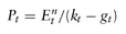
Investors commonly employ cash flow discount models to value equities. Cash flows can be specified in terms of dividends, free cash flow, earnings, and so forth. For example, a simple constant-growth earnings discount model specifies the price of a security at time t as:

(3.1)

where:

P_t = Price of a security at time t

= Expected earnings per share for period n at time t (for example, expected earnings for next fiscal year at time t)
k_t = expected rate of return for the security, given the risk associ ated with it, at time t (also referred to as the discount rate)
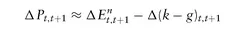
g_t = Long-term (steady-state) expected growth in earnings at time t

Rearranging Equation 3.1 provides the following approximation for change in price levels, which is the variable of interest.

(3.2)

where:

ΔP_t,t + 1 = Change in price between time t and t + 1
Δ

= Change in expected earnings per share for period n between time t and t + 1 (for example, change in next fiscal year earnings between time t and t + 1)
Δ(k - g)_t,t+1= Changein the difference between the discount rate and the long-term expected growth in earnings between time t and t + 1

Furthermore, from Equation 3.1 we can specify the earnings-price (E/P) ratio as:

(3.3)

The change in the E/P ratio is then defined as:

(3.4)

Substituting Equation 3.4 in Equation 3.2 we get:

or

(3.5)

Equation 3.5 stipulates that security returns are fundamentally driven by change in consensus short-term earnings expectation and change in val uation. The change in valuation component of price return is, in turn, a function of the change in the difference between the consensus estimate of the discount rate and the consensus expected long-term earnings growth rate.

Driver #1: Change in Expectation

Equation 3.5 tells us that price changes are driven primarily by how consensus earnings estimates for a given short-term future earnings horizon change over time, rather than by growth in actual earnings. To make this important point clear, let us assume that, for a given stock at time t, the past 12-month realized earnings are $5 per share and the consensus expectation for next fiscal year earnings is $6 per share. At time t + 1, the past 12-month realized earnings are $5 and the consensus expectation for next fiscal year earnings is $9. The growth in 12-month realized earnings is 0 percent. The change in consensus expectation for next fiscal year earnings, the same look-ahead period at each point in time, is +50 percent between time t and t + 1. Equation 3.5 states that this +50 percent change in consensus expectation is one driver of price changes.

Driver #2: Change in Valuation

The other driver is change in valuation (pri...

Table of contents

• Title Page
• Copyright Page
• Dedication
• Foreword
• Preface
• Acknowledgements
• SECTION One - Background
• SECTION Two - ActiveBeta Conceptual Framework
• SECTION Three - ActiveBeta Indexes
• SECTION Four - ActiveBeta Customizable Solutions
• Disclosures
• Bibliography
• About the Authors
• Index