Impedance Spectroscopy

Applications to Electrochemical and Dielectric Phenomena

Vadim F. Lvovich

• Publisher: Wiley
• Year: 2015
• Print ISBN: 9780470627785
• eBook ISBN: 9781118164099
• Edition: 1
• Topic: Physical Sciences
• Subtopic: Physical & Theoretical Chemistry

This book presents a balance of theoretical considerations and practical problem solving of electrochemical impedance spectroscopy. This book incorporates the results of the last two decades of research on the theories and applications of impedance spectroscopy, including more detailed reviews of the impedance methods applications in industrial colloids, biomedical sensors and devices, and supercapacitive polymeric films. The book covers all of the topics needed to help readers quickly grasp how to apply their knowledge of impedance spectroscopy methods to their own research problems. It also helps the reader identify whether impedance spectroscopy may be an appropriate method for their particular research problem. This includes understanding how to correctly make impedance measurements, interpret the results, compare results with expected previously published results form similar chemical systems, and use correct mathematical formulas to verify the accuracy of the data.

Unique features of the book include theoretical considerations for dealing with modeling, equivalent circuits, and equations in the complex domain, review of impedance instrumentation, best measurement methods for particular systems and alerts to potential sources of errors, equations and circuit diagrams for the most widely used impedance models and applications, figures depicting impedance spectra of typical materials and devices, extensive references to the scientific literature for more information on particular topics and current research, and a review of related techniques and impedance spectroscopy modifications.

CHAPTER 1

Fundamentals of Electrochemical Impedance Spectroscopy

1.1. Concept of complex impedance

The concept of electrical impedance was first introduced by Oliver Heaviside in the 1880s and was soon afterward developed in terms of vector diagrams and complex numbers representation by A. E. Kennelly and C. P. Steinmetz [1, p. 5]. Since then the technique has gained in exposure and popularity, propelled by a series of scientific advancements in the field of electrochemistry, improvements in instrumentation performance and availability, and increased exposure to an ever-widening range of practical applications.

For example, the development of the double-layer theory by Frumkin and Grahame led to the development of the equivalent circuit (EC) modeling approach to the representation of impedance data by Randles and Warburg. Extended studies of electrochemical reactions coupled with diffusion (Gerisher) and adsorption (Eppelboin) phenomena, effects of porous surfaces on electrochemical kinetics (de Levie), and nonuniform current and potential distribution dispersions (Newman) all resulted in a tremendous expansion of impedance-based investigations addressing these and other similar problems [1]. Along with the development of electrochemical impedance theory, more elaborate mathematical methods for data analysis came into existence, such as Kramers-Kronig relationships and nonlinear complex regression [1, 2]. Transformational advancements in electrochemical equipment and computer technology that have occurred over the last 30 years allowed for digital automated impedance measurements to be performed with significantly higher quality, better control, and more versatility than what was available during the early years of EIS. One can argue that these advancements completely revolutionized the field of impedance spectroscopy (and in a broader sense the field of electrochemistry), allowing the technique to be applicable to an exploding universe of practical applications. Some of these applications, such as dielectric spectroscopy analysis of electrical conduction mechanisms in bulk polymers and biological cell suspensions, have been actively practiced since the 1950s [3, 4]. Others, such as localized studies of surface corrosion kinetics and analysis of the state of biomedical implants, have come into prominence only relatively recently [5, 6, 7, 8].

In spite of the ever-expanding use of EIS in the analysis of practical and experimental systems, impedance (or complex electrical resistance, for a lack of a better term) fundamentally remains a simple concept. Electrical resistance R is related to the ability of a circuit element to resist the flow of electrical current. Ohm’s Law (Eq. 1-1) defines resistance in terms of the ratio between input voltage V and output current I:

(1-1)

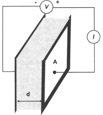
While this is a well-known relationship, its use is limited to only one circuit element—the ideal resistor. An ideal resistor follows Ohm’s Law at all current, voltage, and AC frequency levels. The resistor’s characteristic resistance value R [ohm] is independent of AC frequency, and AC current and voltage signals though the ideal resistor are “in phase” with each other. Let us assume that the analyzed sample material is ideally homogeneous and completely fills the volume bounded by two external current conductors (“electrodes”) with a visible area A that are placed apart at uniform distance d, as shown in Figure 1-1. When external voltage V is applied, a uniform current I passes through the sample, and the resistance is defined as:

FIGURE 1-1 Fundamental impedance experiment

(1-2)

where ρ [ohm cm] is the characteristic electrical resistivity of a material, representing its ability to resist the passage of the current. The inverse of resistivity is conductivity σ [1 / (ohm cm)] or [Sm/cm], reflecting the material’s ability to conduct electrical current between two bounding electrodes.

An ideal resistor can be replaced in the circuit by another ideal element that completely rejects any flow of current. This element is referred as an “ideal” capacitor (or “inductor”), which stores magnetic energy created by an applied electric field, formed when two bounding electrodes are separated by a non-conducting (or “dielectric”) medium. The AC current and voltage signals though the ideal capacitor are completely “out of phase” with each other, with current following voltage. The value of the capacitance presented in Farads [F] depends on the area of the electrodes A, the distance between the electrodes d, and the properties of the dielectric medium reflected in a “relative permittivity” parameter ε as:

(1-3)

where ε₀ = constant electrical permittivity of a vacuum (8.85 10⁻¹⁴F/cm). The relative permittivity value represents a characteristic ability of the analyzed material to store electrical energy. This parameter (often referred to as simply “permittivity” or “dielectric constant”) is essentially a convenient multiplier of the vacuum permittivity constant ε₀ that is equal to a ratio of the material’s permittivity to that of the vacuum. The permittivity values are different for various media: 80.1 (at 20°C) for water, between 2 through 8 for many polymers, and 1 for an ideal vacuum. A typical EIS experiment, where analyzed material characteristics such as conductivity, resistivity, and permittivity are determined, is presented in Figure 1-1.

Impedance is a more general concept than either pure resistance or capacitance, as it takes the phase differences between the input voltage and output current into account. Like resistance, impedance is the ratio between voltage and current, demonstrating the ability of a circuit to resist the flow of electrical current, represented by the “real impedance” term, but it also reflects the ability of a circuit to store electrical energy, reflected in the “imaginary impedance” term. Impedance can be defined as a complex resistance encountered when current flows through a circuit composed of various resistors, capacitors, and inductors. This definition is applied to both direct current (DC) and alternating current (AC).

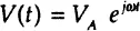
In experimental situations the electrochemical impedance is normally measured using excitation AC voltage signal V with small amplitude V_A (expressed in volts) applied at frequency f (expressed in Hz or 1/sec). The voltage signal V (t), expressed as a function of time t, has the form:

(1-4)

In this notation a “radial frequency” ω of the applied voltage signal (expressed in radians / second) parameter is introduced, which is related to the applied AC frequency f as ω = 2 π f.

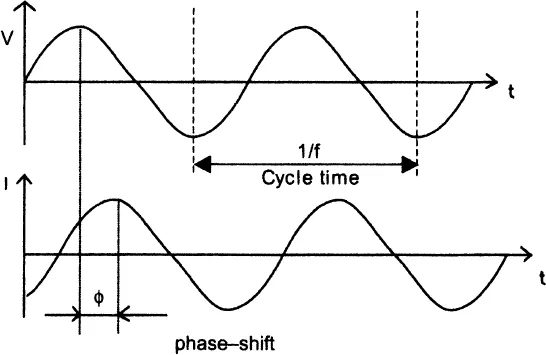
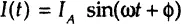
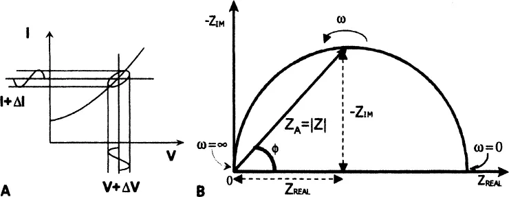
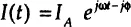
In a linear or pseudolinear system, the current response to a sinusoidal voltage input will be a sinusoid at the same frequency but “shifted in phase” (either forward or backward depending on the system’s characteristics)—that is, determined by the ratio of capacitive and resistive components of the output current (Figure 1-2). In a linear system, the response current signal I(t) is shifted in phase (ϕ) and has a different amplitude, I_A:

FIGURE 1-2 Impedance experiment: sinusoidal voltage input V at a single frequency f and current response I

(1-5)

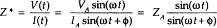
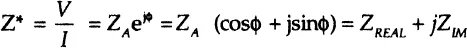
An expression analogous to Ohm’s Law allows us to calculate the complex impedance of the system as the ratio of input voltage V(t) and output measured current I(t):

(1-6)

The impedance is therefore expressed in terms of a magnitude (absolute value), Z_A = |Z|, and a phase shift, ϕ. If we plot the applied sinusoidal voltage signal on the x-axis of a graph and the sinusoidal response signal I(t) on the y-axis, an oval known as a “Lissajous figure” will appear (Figure 1-3A). Analysis of Lissajous figures on oscilloscope screens was the accepted method of impedance measurement prior to the availability of lock-in amplifiers and frequency response analyzers. Modern equipment allows automation in applying the voltage input with variable frequencies and collecting the output impedance (and current) responses as the frequency is scanned from very high (MHz-GHz) values where timescale of the signal is in micro- and nanoseconds to very low frequencies (μHz) with timescales of the order of hours.

FIGURE 1-3 Impedance data representations: A. Lissajous figure; B. Complex impedance plot

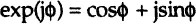
Using Euler’s relationship:

(1-7)

it is possible to express the impedance as a complex function. The potential V(t) is described as:

(1-8)

and the current response as:

(1-9)

The impedance is then represented as a complex number that can also be expressed in complex mathematics as a combination of “real,” or in-phase (Z_REAL), and “imaginary,” or out-of-phase (Z_IM), parts (Figure 1-3B):

(1-10)

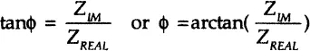
and the phase angle ϕ at a chosen radial frequency ω is a ratio of the imaginary and real impedance components:

(1-11)

1.2. Complex dielectric, modulus, and impedance data representations

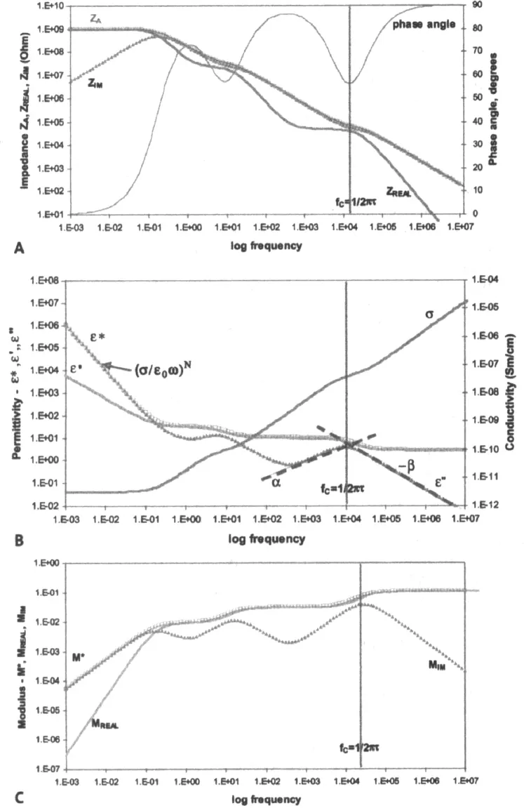
In addition to the AC inputs such as voltage amplitude V_A and radial frequency ω, impedance spectroscopy also actively employs DC voltage modulation (which is sometimes referred to as “offset voltage” or “offset electrochemical potential”) as an important tool to study electrochemical processes. Alternative terms, such as “dielectric spectroscopy” or “modulus spectroscopy,” are often used to describe impedance analysis that is effectively conducted only with AC modulation in the absence of a DC offset voltage (Figure 1-4).

FIGURE 1-4 Representations of complex impedance data as function of AC frequency: A. impedance and phase angle; B. permittivity and conductivity; C. modulus

Dielectric analysis measures two fundamental characteristics of a material—permittivity ε and conductivity σ (or resistivity ρ)—as functions of time, temperature, and AC radial frequency ω. As was discussed above, permittivity and conductivity are two parameters characteristic of respective abilities of analyzed material to store electrical energy and transfer electric charge. Both of these parameters are related to molecular activity. For example, a “dielectric” is a material whose capacitive current (out of phase) exceeds its resistive (in phase) current. An “ideal dielectric” is an insulator with no free charges that is capable of storing electrical energy. The Debye Equation (Eq. 1-12) relates the relative permittivity ε to a concept of material polarization density P [C/m²], or electrical dipole moment [C/m] per unit volume [m³], and the applied electric field V:

(1-12)

Depending on the investigated material and the frequency of the applied electric field, determined polarization can be electronic and atomic (very small translational displacement of the electronic cloud in THz frequency range), orientational or dipolar (rotational moment experienced by permanently polar molecules in kHz-MHz frequency range), and ionic (displacement of ions with respect to each other in Hz-kHz frequency region).

The dielectric analysis typically presents the permittivity and conductivity material properties as a combined “complex permittivity” ε* parameter, which is analogous to the concept of complex impedance Z* (Figure 1-4A). Just as complex impedance can be represented by its real and imaginary components, complex permittivity is a function of two parameters—“real” permittivity (often referred to as “permittivity” or “dielectric constant”) ε’ and imaginary permittivity (or “loss factor”) ε” as:

(1-13)

In dielectric material ε’ represents the alignment of dipoles, which is the energy storage component that is an inverse equivalent of Z_IM. ε” represents the ionic conduction component that is an inverse equivalent of Z_REAL. Both real permittivity and loss factor can be...

Table of contents

• Cover
• Half Title page
• Title page
• Copyright page
• Preface
• Chapter 1: Fundamentals of Electrochemical Impedance Spectroscopy
• Chapter 2: Graphical Representation of Impedance Spectroscopy Data
• Chapter 3: Equivalent Circuits Modeling of the Impedance Phenomenon
• Chapter 4: Examples of Simple Equivalent Circuit Models
• Chapter 5: Impedance Representation of Bulk Material and Electrode Processes
• Chapter 6: Distributed Impedance Models
• Chapter 7: Impedance Analysis of Complex Systems
• Chapter 8: Impedance Instrumentation, Testing, and Data Validation
• Chapter 9: Selected Examples of EIS Applications: Impedance of Electroactive Polymer Films
• Chapter 10: Selected Examples of EIS Analysis Applications: Industrial Colloids and Lubricants
• Chapter 11: EIS Analysis Applications: Cell Suspensions, Protein Adsorption, and Implantable Biomedical Devices
• Chapter 12: Selected Examples of Impedance-Analysis Applications
• Chapter 13: EIS Modifications
• Chapter 14: Conclusions and Perspectives of EIS
• Abbreviations and Symbols
• Index