Ordinary Differential Equations

Michael D. Greenberg

• Publisher: Wiley
• Year: 2014
• Print ISBN: 9781118230022
• eBook ISBN: 9781118243404
• Edition: 1
• Topic: Mathematics
• Subtopic: Applied Mathematics
• Index: Mathematics

Features a balance between theory, proofs, and examples and provides applications across diverse fields of study

Ordinary Differential Equations presents a thorough discussion of first-order differential equations and progresses to equations of higher order. The book transitions smoothly from first-order to higher-order equations, allowing readers to develop a complete understanding of the related theory.

Featuring diverse and interesting applications from engineering, bioengineering, ecology, and biology, the book anticipates potential difficulties in understanding the various solution steps and provides all the necessary details. Topical coverage includes:

• First-Order Differential Equations

• Higher-Order Linear Equations

• Applications of Higher-Order Linear Equations

• Systems of Linear Differential Equations

• Laplace Transform

• Series Solutions

• Systems of Nonlinear Differential Equations

In addition to plentiful exercises and examples throughout, each chapter concludes with a summary that outlines key concepts and techniques. The book's design allows readers to interact with the content, while hints, cautions, and emphasis are uniquely featured in the margins to further help and engage readers.

Written in an accessible style that includes all needed details and steps, Ordinary Differential Equations is an excellent book for courses on the topic at the upper-undergraduate level. The book also serves as a valuable resource for professionals in the fields of engineering, physics, and mathematics who utilize differential equations in their everyday work.

 

An Instructors Manual is available upon request. Email [email protected] for information. There is also a Solutions Manual available. The ISBN is 9781118398999.

Chapter 1

First-Order Differential Equations

1.1 MOTIVATION AND OVERVIEW

1.1.1 Introduction

Typically, phenomena in the natural sciences can be described, or “modeled,” by equations involving derivatives of one or more unknown functions. Such equations are called differential equations.

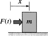
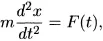
To illustrate, consider the motion of a body of mass m that rests on an idealized frictionless table and is subjected to a force F(t) where t is the time (Fig. 1). According to Newton’s second law of motion, we have

Figure 1. The motion of a mass on a frictionless table subjected to a force F(t).

(1)

in which x(t) is the mass’s displacement. If we know the displacement history x(t) and wish to determine the force F(t) required to produce that displacement, the solution is simple: According to (1), merely differentiate the given x(t) twice and multiply the result by m.

However, if we know the applied force F(t) and wish to determine the displacement x(t) that results, then we say that (1) is a “differential equation” governing the unknown function x(t) because it involves derivatives of x(t) with respect to t. Here, t is the independent variable and x is the dependent variable. The question is: What function or functions x(t), when differentiated twice with respect to t and then multiplied by m (which is a constant), give the prescribed function F(t)?

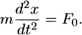
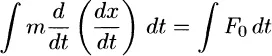
To solve (1) for x(t) we need to undo the differentiations; that is, we need to integrate (1) twice. To illustrate, suppose F(t) = F₀ is a constant, so

(2)

From the calculus,

plus an arbitrary constant.

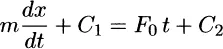
Integrating (2) once with respect to t gives

or

(3)

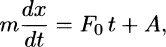
in which C₁ and C₂ are the arbitrary constants of integration. Equivalently,

(4)

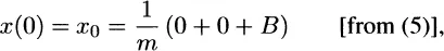
in which the combined constant A = C₂ – C₁ is arbitrary. Integrating again gives mx = F₀t²/2 + At + B, so

(4)

It is a good habit to express the functional dependence explicitly, as we did in (5) when we wrote x(t) instead of just x.

We say that a function is a solution of a given differential equation, on an interval of the independent variable, if its substitution into the equation reduces that equation to an identity everywhere on that interval. If so, we say that the function satisfies the differential equation on that interval. Accordingly, (5) is a solution of (2) on the interval –∞ < t < ∞ because if we substitute it into (2) we obtain F₀ = F₀, which is true for all t.

Actually, (5) is a whole “family” of solutions because A and B are arbitrary. Each choice of A and B in (5) gives one member of that family. That may sound confusing, for weren’t we expecting to find “the” solution, not a whole collection of solutions? What’s missing is that we haven’t specified “starting conditions,” for how can we expect to fully determine the ensuing motion x(t) if we don’t specify how it starts, namely, the displacement and velocity at the starting time t = 0? If we specify those values, say x(0) = x′ and x′ (0) = x′₀ where x₀ and x′₀ are prescribed numbers, then the problem becomes

(6a)

(6b)

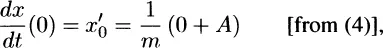
rather than consisting only of the differential equation (2). We seek a function or functions x(t) that satisfy the differential equation md²x/dt² = F₀ on the interval 0 < t < ∞ as well as the conditions x(0) = x₀ and

. We call (6b) initial conditions, and since the problem (6) includes one or more initial conditions we call it an initial value problem or IVP. Application of the initial conditions to the solution (5) gives

Initial value problem is often abbreviated as IVP.

(7a)

(7b)

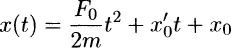
so A = mx′₀ and B = mx₀, and we have the solution

(8)

of (6). Thus, from the differential equation (6a), which is a statement of Newton’s second law, and the initial conditions (6b), we’ve been able to predict the displacement history x(t) for all t > 0.

Whereas the differential equation (2), by itself, has the whole family of solutions given by (5), there is only one within that family that also satisfies the initial conditions (6b), the solution given by (8).

Unfortunately, most differential equations cannot be solved that readily, merely by undoing the derivatives by integration. For instance, suppose the mass is restrained by an ordinary coil spr...

Table of contents

• Cover
• Contents
• Title Page
• Copyright
• Preface
• CHAPTER 1: FIRST-ORDER DIFFERENTIAL EQUATIONS
• CHAPTER 2: HIGHER-ORDER LINEAR EQUATIONS
• CHAPTER 3: APPLICATIONS OF HIGHER-ORDER EQUATIONS
• CHAPTER 4: SYSTEMS OF LINEAR DIFFERENTIAL EQUATIONS
• CHAPTER 5: LAPLACE TRANSFORM
• CHAPTER 6: SERIES SOLUTIONS
• CHAPTER 7: SYSTEMS OF NONLINEAR DIFFERENTIAL EQUATIONS
• APPENDIX A: REVIEW OF PARTIAL FRACTION EXPANSIONS
• APPENDIX B: REVIEW OF DETERMINANTS
• APPENDIX C: REVIEW OF GAUSS ELIMINATION
• APPENDIX D: REVIEW OF COMPLEX NUMBERS AND THE COMPLEX PLANE
• ANSWERS TO EXERCISES
• INDEX