Statistics for Censored Environmental Data Using Minitab and R

Dennis R. Helsel

• Publisher: Wiley
• Year: 2011
• Print ISBN: 9780470479889
• eBook ISBN: 9781118162767
• Edition: 2
• Topic: Mathematics
• Subtopic: Probability & Statistics
• Index: Mathematics

Praise for the First Edition

"... an excellent addition to an upper-level undergraduate course on environmental statistics, and... a 'must-have' desk reference for environmental practitioners dealing with censored datasets."
—Vadose Zone Journal

Statistics for Censored Environmental Data Using Minitab ® and R, Second Edition introduces and explains methods for analyzing and interpreting censored data in the environmental sciences. Adapting survival analysis techniques from other fields, the book translates well-established methods from other disciplines into new solutions for environmental studies.

This new edition applies methods of survival analysis, including methods for interval-censored data to the interpretation of low-level contaminants in environmental sciences and occupational health. Now incorporating the freely available R software as well as Minitab ® into the discussed analyses, the book features newly developed and updated material including:

• A new chapter on multivariate methods for censored data
• Use of interval-censored methods for treating true nondetects as lower than and separate from values between the detection and quantitation limits ("remarked data")
• A section on summing data with nondetects
• A newly written introduction that discusses invasive data, showing why substitution methods fail
• Expanded coverage of graphical methods for censored data

The author writes in a style that focuses on applications rather than derivations, with chapters organized by key objectives such as computing intervals, comparing groups, and correlation. Examples accompany each procedure, utilizing real-world data that can be analyzed using the Minitab ® and R software macros available on the book's related website, and extensive references direct readers to authoritative literature from the environmental sciences.

Statistics for Censored Environmental Data Using Minitab ® and R, Second Edition is an excellent book for courses on environmental statistics at the upper-undergraduate and graduate levels. The book also serves as a valuable reference for??environmental professionals, biologists, and ecologists who focus on the water sciences, air quality, and soil science.

Chapter 1

Things People Do with Censored Data that Are Just Wrong

Censored observations are low-level concentrations of organic or inorganic chemicals with values known only to be somewhere between zero and the laboratory's detection/reporting limits. The chemical signal on the measuring instrument is small in relation to the process noise. Measurements are considered too imprecise to report as a single number, so the value is commonly reported as being less than an analytical threshold, for example, “<1.” Long considered second-class data, censored observations complicate the familiar computations of descriptive statistics, of testing differences among groups, and of correlation coefficients and regression equations.

Statisticians use the term “censored data” for observations that are not quantified, but are known only to exceed or to be less than a threshold value. Values known only to be below a threshold (less-thans) are left-censored data. Values known only to exceed a threshold (greater-thans) are right-censored data. Values known only to be within an interval (between 2 and 5) are interval-censored data. Techniques for computing statistics for censored data have long been employed in medical and industrial studies, where the length of time is measured until an event occurs, such as the recurrence of a disease or failure of a manufactured part. For some observations the event may not have occurred by the time the experiment ends. For these, the time is known only to be greater than the experiment's length, a right-censored “greater-than” value. Methods for incorporating censored data when computing descriptive statistics, testing hypotheses, and performing correlation and regression are all commonly used in medical and industrial statistics, without substituting arbitrary values. These methods go by the names of “survival analysis” (Klein and Moeschberger, 2003) and “reliability analysis” (Meeker and Escobar, 1998). There is no reason why these same methods should also not be used in the environmental sciences, but until recently their use has been relatively rare. Environmental scientists have not often been trained in survival analysis methods.

The worst practice when dealing with censored observations is to exclude or delete them. This produces a strong bias in all subsequent measures of location or hypothesis tests. After excluding the 80% of observations that are left-censored nondetects, for example, the mean of the top 20% of concentrations is reported. This provides almost no insight into the original data. Excluding censored observations removes the primary information contained in them—the proportion of data in each group that lies below the reporting limit(s). And while better than deleting censored observations, fabricating artificial values as if these had been measured provides its own inaccuracies. Fabrication (substitution) adds an invasive signal to the data that was not previously there, potentially obscuring the information present in the measured observations.

Studies 25 years ago found substitution to be a poor method for computing descriptive statistics (Gilliom and Helsel, 1986). Numerous subsequent articles (see Chapter 6) have reinforced that opinion. Justifications for using one-half the reporting limit usually point back to Hornung and Reed (1990), who only considered estimation of the mean, and assumed that data below the single reporting limit follow a uniform distribution. Estimating the mean is not the primary issue. Any substitution of a constant fraction times the reporting limits will distort estimates of the standard deviation, and therefore all (parametric) hypothesis tests using that statistic. This is illustrated in a later section using simulations. Also, justifications for substitution rarely consider the common occurrence of changing reporting limits. Reporting limits change over time due to methods changes, change between samples due to changing interferences, amounts of sample submitted, and other causes. Substituting values that are tied to changing reporting limits introduces an external (exotic) signal into the data that was not present in the media sampled. Substituted values using a fraction anywhere between 0 and 0.99 times the detection limit are equivalently arbitrary, easy, and wrong.

There have been voices objecting to substitution. In 1967, a US Geological Survey report by Miesch (1967) stated that substituting a constant for censored observations created unnecessary errors, instead recommending Cohen's Maximum Likelihood procedure. Cohen's procedure was published in the statistical literature in the late 1950s and early 1960s (Cohen, 1957, 1961), so its movement into an applied field by 1967 is a credit indeed to Miesch. Two other early environmental pioneers of methods for censored data are Millard and Deverel (1988) and Farewell (1989). Millard and Deverel (1988) pioneered the use of two-group survival analysis methods in environmental work, testing for differences in metals concentrations in the groundwaters of two aquifers. Many censored values were present, at multiple reporting limits. They found differences in zinc concentrations between the two aquifers using a survival analysis method called a score test (see Chapter 9). Had they substituted one-half the reporting limit for zinc concentrations and run a t-test, they would not have found those differences. Farewell (1989) suggested using nonparametric survival analysis techniques for estimating descriptive statistics, hypothesis testing, and regression for censored water quality data. Many of his suggestions have been expanded in the pages of this book. Since that time, a guide to the use of censored data techniques for environmental studies was published by Akritas (1994) as a chapter in volume 12 of the Handbook of Statistics. In an applied setting, She (1997) computed descriptive statistics of organics concentrations in sediments using a survival analysis method called Kaplan–Meier. Means, medians, and other statistics were computed without substitutions, even though 20% of data were observations censored at eight different reporting limits.

Guidance documents have evolved over the years when recommending methods to deal with censored observations. In 1991 the Technical Support Document for Water-Quality Based Toxics Control (USEPA, 1991) recommended use of the delta-lognormal (also called Aitchison's or DLOG) method when computing means for censored data. Gilliom and Helsel (1986) had previously shown that the delta-lognormal method was essentially the same as substituting zeros for censored observations, and so its estimated mean was consistently biased low. Hinton (1993) found that the delta-lognormal method was biased low and had a larger bias than either Cohen's MLE or the parametric ROS procedure (see Chapter 6 for more information on the latter). The 1998 Guidance for data quality assessment: Practical methods for data analysis recommended substitution when there were fewer than 15% censored observations, otherwise using Cohen's method (USEPA, 1998a). Cohen's method, an approximate MLE method using a lookup table valid for only one reporting limit, may have been innovative when proposed by Miesch in 1967, but by 1998 there were better methods available. Minnesota's Data Analysis Protocol for the Ground Water Monitoring and Assessment Program presented an early adoption of some of the better, simpler methods for censored data (Minnesota Pollution Control Agency, 1999). In 2002, substitution of the reporting limit was still recommended in the Development Document for theProposed Effluent Limitations Guidelines and Standards for the Meat and Poultry Products Industry Point Source Category (USEPA, 2002c). States have forged their own way at times—in 2005 the California Ocean Plan recommended use of robust ROS when computing a mean and upper confidence limit on the mean (UCL95) for determining reasonable potential (California EPA, 2005, Appendix VI). More recently, the 2009 Stormwater BMP Monitoring Manual (Geosyntec Consultants and Wright Water Engineers, 2009) states “It is strongly recommended that simple substitution is avoided,” and instead recommends methods found in this book for estimating summary statistics. And the 2009 Unified Guidance on statistical methods for groundwater quality at RCRA facilities (USEPA, 2009) recommended the use of survival analysis methods, although they unfortunately allowed substitution for estimation and hypothesis testing when the proportion of censored observations was below 15%.

1.1 Why Not Substitute—Missing the Signals that Are Present in the Data

Statisticians generate simulated data for much the same reasons as chemists prepare standard solutions—so that the starting conditions are exactly known. Statistical methods are then applied to the data, and the similarity of their results to the known, correct values provides a measure of the quality of each method. Fifty pairs of X,Y data were generated by Helsel (2006) with X values uniformly distributed from 0 to 100. The Y values were computed from a regression equation with slope = 1.5 and intercept = 120. Noise was then randomly added to each Y value so that points did not fall exactly on the straight line. The result is data having a strong linear relation between Y and X with a moderate amount of noise in comparison to that linear signal.

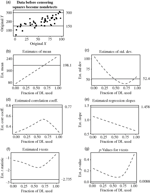
The noise applied to the data represented a “mixed normal” distribution, two normal distributions where the second had a larger standard deviation than the first. All of the added noise had a mean of zero, so the expected result over many simulations is still a linear relationship between X and Y with a slope = 1.5 and intercept = 120. Eighty percent of data came from the distribution with the smaller standard deviation, while 20% reflected the second distribution's increased noise level, to generate outliers. The 50 generated values are plotted in Figure 1.1a.

Figure 1.1 (a) Data used. Horizontal lines are reporting limits. (b–g) Estimated values for statistics of censored data Y) as a function of the fraction of the detection limit (X) used to substitute values for each nondetect. As an example, 0.5 corresponds to substitution of one-half the detection limit for all censored values. Horizontal lines are at target values of each statistic obtained using uncensored values.

The 50 observations were also assigned to one of the two groups in a way that group differences should be discernible. The first group is mostly of early (low X) data and second of later (high X) data. The mean, standard deviation, correlation coefficient, regression slope of Y versus X, a t-test between the means of the two groups, and its p-value for the 50 generated observations in Figure 1.1a were then all computed and stored. These “benchmark” statistics are the target values to which later estimates are compared. The later estimates are made after censoring the points plotted as squares in Figure 1.1a.

Two reporting limits (at 150 and 300) were then applied to the data, the black dots of Figure 1.1a remaining as uncensored values with unique numbers, and the squares becoming censored observations below one of the two reporting limits. In total, 33 of 50 observations, or 66% of observations, were censored below one of the two reporting limits. This is within the range of amounts of censoring found in many environmental studies. Use of a smaller percent censoring would produce many of the same effects as found here, though not as obvious or as strong. All of the data between 150 and the higher reporting limit of 300 were censored as <300. In order to mimic laboratory results with two reporting limits, data below 150 were randomly selected and some assigned <150 while others became <300.

1.1.1 Results

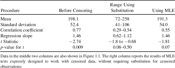
Figure 1.1b–g illustrate the results of estimating a statistic or running a hypothesis test after substituting numbers for censored observations by multiplying the reporting limit value by a fraction between 0 and 1. Estimated values for each statistic are plotted on the Y-axes, with the fraction of the reporting limit used in substitution on the X-axes. A fraction of 0.5 on the X axis corresponds to substituting a value of 75 for all <150s, and 150 for all <300s, for example. On each plot is also shown the value for that statistic before censoring, as a “benchmark” horizontal line. The same information is presented in tabular form in Table 1.1.

Table 1.1 Statistics and Test Results Before and After Censoring.

Estimates of the mean of Y are presented in Figure 1.1b. The mean Y before censoring equals 198.1. Afterwards, substitution across the range between 0 and the detection limits (DL) produces a mean Y that can fall anywhere between 72 and 258. For this data set, substituting data using a fraction somewhere around 0.7 DL appears to mimic the uncensored mean. But for another data set with different characteristics, another fraction might be “best.” And 0.7 is not the “best” for these data to duplicate the uncensored standard deviation, as shown in Figure 1.1c. Something larger or smaller, closer to 0.5 or 0.9 would work better for that statistic, for this set of data. Performance will also differ depending on the proportion of data censored, as discussed later. Results for the median (not shown) were similar to those for the mean, and results for the interquartile range (not shown) were similar to those for t...

Table of contents

• Cover
• Wiley Series in Statistics in Practice
• Title Page
• Copyright
• Preface
• Acknowledgments
• Introduction to the First Edition: An Accident Waiting To Happen
• Introduction to the Second Edition: Invasive Data
• Chapter 1: Things People Do with Censored Data that Are Just Wrong
• Chapter 2: Three Approaches for Censored Data
• Chapter 3: Reporting Limits
• Chapter 4: Reporting, Storing, and Using Censored Data
• Chapter 5: Plotting Censored Data
• Chapter 6: Computing Summary Statistics and Totals
• Chapter 7: Computing Interval Estimates
• Chapter 8: What Can be Done When All Data Are Below the Reporting Limit?
• Chapter 9: Comparing Two Groups
• Chapter 10: Comparing Three or More Groups
• Chapter 11: Correlation
• Chapter 12: Regression and Trends
• Chapter 13: Multivariate Methods for Censored Data
• Chapter 14: The NADA for R Software
• Appendix: Datasets
• References
• Index
• Statistics in Practice