Introduction to Finite Element Analysis

Formulation, Verification and Validation

Barna Szabó, Ivo Babuška

• Publisher: Wiley
• Year: 2011
• Print ISBN: 9780470977286
• eBook ISBN: 9781119993483
• Edition: 1
• Topic: Technology & Engineering
• Subtopic: Technology & Engineering Research & Skills
• Index: Technology & Engineering

When using numerical simulation to make a decision, how can its reliability be determined? What are the common pitfalls and mistakes when assessing the trustworthiness of computed information, and how can they be avoided?

Whenever numerical simulation is employed in connection with engineering decision-making, there is an implied expectation of reliability: one cannot base decisions on computed information without believing that information is reliable enough to support those decisions. Using mathematical models to show the reliability of computer-generated information is an essential part of any modelling effort.

Giving users of finite element analysis (FEA) software an introduction to verification and validation procedures, this book thoroughly covers the fundamentals of assuring reliability in numerical simulation. The renowned authors systematically guide readers through the basic theory and algorithmic structure of the finite element method, using helpful examples and exercises throughout.

• Delivers the tools needed to have a working knowledge of the finite element method
• Illustrates the concepts and procedures of verification and validation
• Explains the process of conceptualization supported by virtual experimentation
• Describes the convergence characteristics of the h-, p- and hp-methods
• Covers the hierarchic view of mathematical models and finite element spaces
• Uses examples and exercises which illustrate the techniques and procedures of quality assurance
• Ideal for mechanical and structural engineering students, practicing engineers and applied mathematicians
• Includes parameter-controlled examples of solved problems in a companion website ( www.wiley.com/go/szabo )

1

Introduction

Engineering decision-making processes increasingly rely on information computed from approximate solutions of mathematical models. Engineering decisions have legal and ethical implications. The standard applied in legal proceedings in civil cases in the United States is to have opinions, recommendations and decisions “based upon a reasonable degree of engineering certainty.” Codes of ethics of engineering societies impose higher standards. For example, the Code of Ethics of the Institute of Electrical and Electronics Engineers (IEEE) requires members “to accept responsibility in making engineering decisions consistent with the safety, health, and welfare of the public, and to disclose promptly factors that might endanger the public or the environment” and “to be honest and realistic in stating claims or estimates based on available data.”

An important challenge facing the computational engineering community is to establish procedures for creating evidence that will show, with a high degree of certainty, that a mathematical model of some physical reality, formulated for a particular purpose, can in fact represent the physical reality in question with sufficient accuracy to make predictions based on mathematical models useful and justifiable for the purposes of engineering decision-making and the errors in the numerical approximation are sufficiently small. There is a large and rapidly growing body of work on this subject. See, for example, [38a], [68], [52], [51], [99]. The formulation and numerical treatment of mathematical models for use in support of engineering decision-making in the field of solid mechanics is addressed in a document issued by the American Society of Mechanical Engineers (ASME) and adopted by the American National Standards Institute (ANSI) [33]. The Simulation Interoperability Standards Organization (SISO) is another important source of information.

The considerations underlying the selection of mathematical models and methods for the estimation and control of modeling errors and the errors of discretization are the two main topics of this book. In this chapter a brief overview is presented and the basic terminology is introduced.

1.1 Numerical simulation

The goal of numerical simulation is to make predictions concerning the response of physical systems to various kinds of excitation and, based on those predictions, make informed decisions. To achieve this goal, mathematical models are defined and the corresponding numerical solutions are computed. Mathematical models should be understood to be idealized representations of reality and should never be confused with the physical reality that they are supposed to represent.

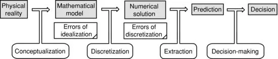
The choice of a mathematical model depends on its intended use: What aspects of physical reality are of interest? What data must be predicted? What accuracy is required? The main elements of numerical simulation and the associated errors are indicated schematically in Figure 1.1.

Figure 1.1 The main elements of numerical simulation and the associated errors.

Some errors are associated with the mathematical model and some errors are associated with its numerical solution. These are called errors of idealization and errors of discretization respectively. For the predictions to be reliable both kinds of errors have to be sufficiently small. The errors of idealization are also called modeling errors. Conceptualization is a process by which a mathematical model is formulated. Discretization is a process by which the exact solution of the mathematical model is approximated. Extraction is a process by which the data of interest are computed from the approximate solution. Some authors refer to the data of interest by the term “system response quantities” (SRQs).

1.1.1 Conceptualization

Mathematical models are operators that transform one set of data, the input, into another set, the output. In solid mechanics, for example, one is typically interested in predicting displacements, strains and stresses, stress intensity factors, limit loads, natural frequencies, etc., given a description of the solution domain, constitutive equations and boundary conditions (loading and constraints). Common to all models are the equations that represent the conservation of momentum (in static problems the equations of equilibrium), the strain–displacement relations and constitutive laws.

The end product of conceptualization is a mathematical model. The definition of a mathematical model involves specification of the following:

1. Theoretical formulation. The applicable physical laws, together with certain simplifications, are stated as a mathematical problem in the form of ordinary or partial differential equations, or extremum principles. For example, the classical differential equation for elastic beams is derived from the assumptions of the theory of elasticity supplemented by the assumption that the transverse variation of the longitudinal components of the displacement vector can be approximated by a linear function without significantly affecting the data of interest, which are typically the displacements, bending moments, shear forces, natural frequencies, etc.

2. Specification of the input data. The input data comprise the following:

a. Data that characterize the solution domain. In engineering practice solution domains are usually constructed by means of computer-aided design (CAD) tools. CAD tools produce idealized representations of real objects. The details of idealization depend on the choice of the CAD tool and the skills and preferences of its operator.

b. Physical properties (elastic moduli, yield stress, coefficients of thermal expansion, thermal conductivities, etc.)

c. Boundary conditions (loads, constraints, prescribed temperatures, etc.)

d. Information or assumptions concerning the reference state and the initial conditions

e. Uncertainties. When some information needed in the formulation of a mathematical model is unknown then the uncertainty is said to be cognitive (also called epistemic). For example, the magnitude and distribution of residual stresses is usually unknown, some physical properties may be unknown, etc. Statistical uncertainties (also called aleatory uncertainties) are always present. Even when the average values of needed physical properties, loading and other data are known, there are statistical variations, possibly very substantial variations, in these data. Consideration of these uncertainties is necessary for proper interpretation of the computed information.
Various methods are available for accounting for uncertainties. The choice of method depends on the quality and reliability of the available information. One such method, known as the Monte Carlo method, is to characterize input data as random variables and use repeated random sampling to compute their effects on the data of interest. If the probability density functions of the input data are sufficiently accurate and sufficiently large samples are taken then a reasonable estimate of the probability distribution of the data of interest can be obtained.

3. Statement of objectives. Definitions of the data of interest and the corresponding permissible error tolerances.

Conceptualization involves the application of expert knowledge, virtual experimentation and calibration.

Application of expert knowledge

Depending on the intended use of the model and the required accuracy of prediction, various simplifying assumptions are introduced. For example, the assumptions incorporated in the linear theory of elasticity, along with simplifying assumptions concerning the domain and the boundary conditions, are widely used in mechanical and structural engineering applications. In many applications further simplifications are introduced, resulting in beam, plate and shell models, planar models and axisymmetric models, each of which imposes additional restrictions on what boundary conditions can be specified and what data can be computed from the solution.

In the engineering literature the commonly used simplified models are grouped into separate model classes, called theories. For example, various beam, plate and shell theories have been developed. The formulation of these theories typically involves a statement on the assumed mode of deformation (e.g., plane sections remain plane and normal to the mid-surface of a deformed beam), the relationship between the functions that characterize the deformation and the strain tensor (e.g., the strain is proportional to the curvature and the distance from the neutral axis), application of Hooke's law, and statement of the equations of the equilibrium.

In undergraduate engineering curricula each model...

Table of contents

• Cover
• Series
• Title Page
• Copyright
• Dedication
• About the Authors
• Series Preface
• Preface
• 1: Introduction
• 2: An Outline of the Finite Element Method
• 3: Formulation of Mathematical Models
• 4: Generalized Formulations
• 5: Finite Element Spaces
• 6: Regularity and Rates of Convergence
• 7: Computation and Verification of Data
• 8: What should be Computed and Why?
• 9: Beams, Plates and Shells
• 10: Nonlinear Models
• Appendix A: Definitions
• Appendix B: Numerical Quadrature
• Appendix C: Properties of the Stress Tensor
• Appendix D: Computation of Stress Intensity Factors
• Appendix E: Saint-Venant's Principle
• Appendix F: Solutions for Selected Exercises
• Bibliography
• Index