![]()
Chapter 1
Introduction
Biplots have been with us at least since Descartes, if not from the time of Ptolemy who had a method for fixing the map positions of cities in the ancient world. The essential ingredients are coordinate axes that give the positions of points. From the very beginning, the concept of distance was central to the Cartesian system, a point being fixed according to its distance from two orthogonal axes; distance remains central to much of what follows. Descartes was concerned with how the points moved in a smooth way as parameters changed, so describing straight lines, conics and so on. In statistics, we are interested also in isolated points presented in the form of a scatter diagram where, typically, the coordinate axes represent variables and the points represent samples or cases. Cartesian geometry soon developed three-dimensional and then multidimensional forms in which there are many coordinate axes. Although two-dimensional scatter diagrams are invaluable for showing data, multidimensional scatter diagrams are not. Therefore, statisticians have developed methods for approximating multidimensional scatter in two, or perhaps three, dimensions. It turns out that the original coordinate axes can also be displayed as part of the approximation, although inevitably they lose their orthogonality. The essential property of all biplots is the two modes, such as variables and samples. For obvious reasons, we shall be concerned mainly with two-dimensional approximations but should stress at the outset that the bi- of biplots refers to the two modes and not the usual two dimensions used for display.
Biplots, not necessarily referred to by name, have been used in one form or another for many years, especially since computer graphics have become readily available. The term ‘biplot’ is due to Gabriel (1971) who popularized versions in which the variables are represented by directed vectors. Gower and Hand (1996) particularly stressed the advantages of presenting biplots with calibrated axes, in much the same way as for conventional coordinate representations. A feature of this book is the wealth of examples of different kinds of biplots. Although there are many novel ideas in this book, we acknowledge our debts to many others whose work is cited either in the current text or in the bibliography of Gower and Hand (1996).
1.1 Types of Biplots
We may distinguish two main types of biplot:
- asymmetric (biplots giving information on sample units and variables of a data matrix);
- symmetric (biplots giving information on rows and columns of a two-way table).
In symmetric biplots, rows and columns may be interchanged without loss of information, while in asymmetric biplots variables and sample units are different kinds of object that may not be interchanged.
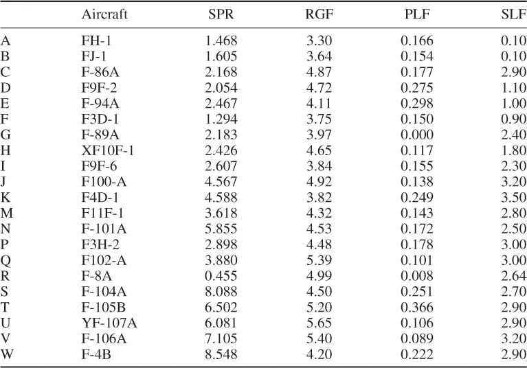
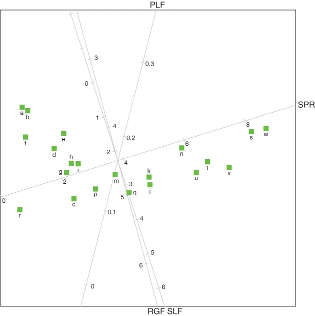
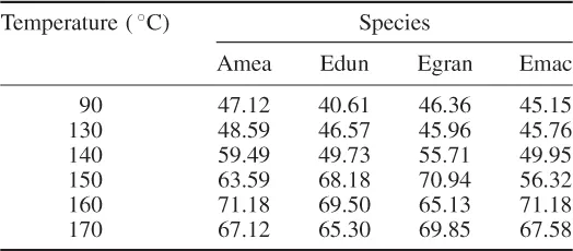
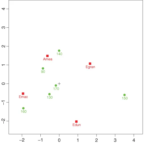
Consider the data on four variables measured on 21 aircraft in Table 1.1. The corresponding biplot in Figure 1.1 represents the 21 aircraft as sample points and the four variables as biplot axes. It will not be sensible to exchange the two sets, representing the aircraft as continuous axes and the variables as points. Next, consider the two-way table in Table 1.2. Exchanging the rows and columns of this table will have no effect on the information contained therein. For such a symmetric data set, both the rows and columns are represented as points as shown in Figure 1.2. Details on the construction of these biplots are deferred to later chapters.
Table 1.1 Values of four variables, SPR (specific power, proportional to power per unit weight), RGF (flight range factor), PLF (payload as a fraction of gross weight of aircraft) and SLF (sustained load factor), for 21 aircraft labelled in column 2. From Cook and Weisberg (1982, Table 2.3.1), derived from 1979 RAND Corporation report.
Table 1.2 Species × Temperature two-way table of percentage cellulose measured in wood pulp from four species after a hot water wash.
We shall see that this distinction between symmetric and asymmetric biplots affects what is permissible in the construction of a biplot. Within this broad classification, other major considerations are:
- the types of variable (quantitative, qualitative, ordinal, etc.);
- the method used for displaying samples (multidimensional scaling and related methods);
- what the biplot display is to be used for (especially for prediction or for interpolation).
The following can be represented in an asymmetric biplot:
- distances between samples;
- relationships between variables;
- inner products between samples and variables.
However, only two of these characteristics can be optimally represented in a single biplot. In the simple biplot in Figure 1.1 all the calibration scales are linear with evenly spaced calibration points. Other types of scale are...