Finite Difference Methods in Financial Engineering

A Partial Differential Equation Approach

Daniel J. Duffy

• Publisher: Wiley
• Year: 2013
• Print ISBN:
  9780470858820
• Edition: 1
• eBook ISBN:
  9781118856482
• Topic: Business
• Subtopic: Finance
• Index: Business

The world of quantitative finance (QF) is one of the fastest growing areas of research and its practical applications to derivatives pricing problem. Since the discovery of the famous Black-Scholes equation in the 1970's we have seen a surge in the number of models for a wide range of products such as plain and exotic options, interest rate derivatives, real options and many others. Gone are the days when it was possible to price these derivatives analytically. For most problems we must resort to some kind of approximate method.

In this book we employ partial differential equations (PDE) to describe a range of one-factor and multi-factor derivatives products such as plain European and American options, multi-asset options, Asian options, interest rate options and real options. PDE techniques allow us to create a framework for modeling complex and interesting derivatives products. Having defined the PDE problem we then approximate it using the Finite Difference Method (FDM). This method has been used for many application areas such as fluid dynamics, heat transfer, semiconductor simulation and astrophysics, to name just a few. In this book we apply the same techniques to pricing real-life derivative products. We use both traditional (or well-known) methods as well as a number of advanced schemes that are making their way into the QF literature:

• Crank-Nicolson, exponentially fitted and higher-order schemes for one-factor and multi-factor options
• Early exercise features and approximation using front-fixing, penalty and variational methods
• Modelling stochastic volatility models using Splitting methods
• Critique of ADI and Crank-Nicolson schemes; when they work and when they don't work
• Modelling jumps using Partial Integro Differential Equations (PIDE)
• Free and moving boundary value problems in QF

Included with the book is a CD containing information on how to set up FDM algorithms, how to map these algorithms to C++ as well as several working programs for one-factor and two-factor models. We also provide source code so that you can customize the applications to suit your own needs.

Part I

The Continuous Theory of Partial Differential Equations

Chapter 1

An Introduction to Ordinary Differential Equations

1.1 INTRODUCTION AND OBJECTIVES

Part I of this book is devoted to an overview of ordinary and partial differential equations. We discuss the mathematical theory of these equations and their relevance to quantitative finance. After having read the chapters in Part I you will have gained an appreciation of one-factor and multi-factor partial differential equations.

In this chapter we introduce a class of second-order ordinary differential equations as they contain derivatives up to order 2 in one independent variable. Furthermore, the (unknown) function appearing in the differential equation is a function of a single variable. A simple example is the linear equation

(1.1)

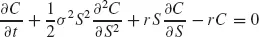
In general we seek a solution u of (1.1) in conjunction with some auxiliary conditions. The coefficients a, b, c and f are known functions of the variable x. Equation (1.1) is called linear because all coefficients are independent of the unknown variable u. Furthermore, we have used the following shorthand for the first- and second-order derivatives with respect to x:

(1.2)

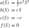
We examine (1.1) in some detail in this chapter because it is part of the Black–Scholes equation

(1.3)

where the asset price S plays the role of the independent variable x and t plays the role of time. We replace the unknown function u by C (the option price). Furthermore, in this case, the coefficients in (1.1) have the special form

(1.4)

In the following chapters our intention is to solve problems of the form (1.1) and we then apply our results to the specialised equations in quantitative finance.

1.2 TWO-POINT BOUNDARY VALUE PROBLEM

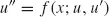
Let us examine a general second-order ordinary differential equation given in the form

(1.5)

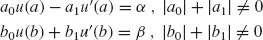
where the function f depends on three variables. The reader may like to check that (1.1) is a special case of (1.5). In general, there will be many solutions of (1.5) but our interest is in defining extra conditions to ensure that it will have a unique solution. Intuitively, we might correctly expect that two conditions are sufficient, considering the fact that you could integrate (1.5) twice and this will deliver two constants of integration. To this end, we determine these extra conditions by examining (1.5) on a bounded interval (a, b). In general, we discuss linear combinations of the unknown solution u and its first derivative at these end-points:

(1.6)

We wish to know the conditions under which problem (1.5), (1.6) has a unique solution. The full treatment is given in Keller (1992), but we discuss the main results in this section. First, we need to place some restrictions on the function f that appears on the right-hand side of equation (1.5).

Definition 1.1. The function f(x, u, v) is called uniformly Lipschitz continuous if

(1.7)

where K is some constant, and x, ut, and v are real numbers.

We now state the main result (taken from Keller, 1992).

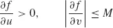
Theorem 1.1. Consider the function f(x; u, v) in (1.5) and suppose that it is uniformly Lipschitz continuous in the region R, defined by:

(1.8)

Suppose, furthermore, that f has continuous derivatives in R satisfying, for some constant M,

(1.9)

and, that

(1.10)

Then the boundary-value problem (1.5), (1.6) has a unique solution.

This is a general result and we can use it in new problems to assure us that they have a unique solution.

1.2.1 Special kinds of boundary condition

The linea...

Table of contents

• Cover
• Half Title page
• Title page
• Copyright page
• Chapter 0: Goals of this Book and Global Overview
• Part I: The Continuous Theory of Partial Differential Equations
• Part II: Finite Difference Methods: the Fundamentals
• Part III: Applying FDM to One-Factor Instrument Pricing
• Part IV: FDM for Multidimensional Problems
• Part V: Applying FDM to Multi-Factor Instrument Pricing
• Part VI: Free and Moving Boundary Value Problems
• Part VII: Design and Implementation in C++
• Appendix 1: An Introduction to Integral and Partial Integro-Differential Equations
• Appendix 2: An Introduction to the Finite Element Method
• Bibliography
• Index